← Experiment

EFT Mean-Gravity Framework vs. the Minimal NFW Baseline for Cold Dark Matter (DM)

Author: Guanglin Tu
Email: riniky@energyfilament.org | ORCID: 0009-0003-7659-6138
Affiliation: EFT Working Group, Shenzhen Energy Filament Science Research Co., Ltd. (China)
Version: v1.1 | Date: 2026-02-14

Preprint (not peer reviewed) | This version is intended for public dissemination and reproducibility, and does not represent the final journal-published version.

License: Report (CC BY-NC-ND 4.0); full reproduction package (CC BY 4.0).

Publication-grade report (Concept DOI): https://doi.org/10.5281/zenodo.18526334 Full reproduction package (Concept DOI): https://doi.org/10.5281/zenodo.18526286

0 Executive Summary

This report is a publication-grade archive edition deposited on Zenodo. It provides an integrated, auditable chain covering data, the model ledger, fair comparison, closure testing, and reproducibility materials. Appendix B (P1A) serves as a robustness supplement. It focuses on stress tests with a “more standard DM baseline + one key lensing systematic,” used to assess the sensitivity of the main conclusions to more realistic DM modeling and lensing-systematics treatment.

Core conclusions (four directly quotable statements; see Section 2.4):

(1) In rotation-curve (RC) fitting, the EFT family significantly outperforms DM_RAZOR under all kernel/prior combinations; a typical improvement is Δlog𝓛_RC ≈ 10^3 (see Table S1a).
(2) In the RC→GGL closure test, EFT shows stronger cross-probe transferability: the closure strength Δlog𝓛_closure (True−Perm) is significantly higher than that of DM_RAZOR, and the difference is robust under covariance shrinkage, R_min, and σ_int scans (see Fig. S3 and Table S1b).
(3) In the joint fit (RC+GGL), EFT retains a stable advantage; under the negative control that breaks the shared mapping, this advantage collapses, supporting the interpretation that the “mean-gravity effect” comes from the shared mapping rather than an accidental fit (see Fig. S4).
(4) Without substantially increasing dimensionality, Appendix B (P1A) stress-tests the DM side with more standard DM baseline modules and one key lensing-systematics nuisance. These enhancements do not remove EFT’s closure advantage (see Table B1 and Fig. B1).

Data and code availability: report Concept DOI 10.5281/zenodo.18526334; full reproduction package Concept DOI 10.5281/zenodo.18526286. The tags corresponding to Appendix B (P1A) are run_tag=20260213_151233, closure_tag=20260213_161731, and joint_tag=20260213_195428.

1 Abstract

We conduct a reproducible quantitative comparison of two theoretical frameworks under the same data and the same statistical protocol: the “mean-gravity correction” model proposed by Energy Filament Theory (EFT; distinct from the common abbreviation for effective field theory), and a baseline cold dark matter (DM) NFW halo model (DM_RAZOR). DM_RAZOR is deliberately chosen as a “minimal DM baseline”: an NFW halo with a fixed c–M relation (without halo-to-halo scatter), serving as an auditable and reproducible control. It should also be emphasized that this paper treats EFT as a phenomenological, MOND-like effective-field/effective-response parameterization for testing under a unified statistical protocol, rather than deriving its microscopic first principles within this work.

The data consist of 2,295 velocity data points from SPARC rotation curves (RC), uniformly preprocessed and binned (104 galaxies, 20 RC bins), together with KiDS-1000 galaxy–galaxy weak-lensing (GGL) excess surface density ΔΣ(R) (4 stellar-mass bins × 15 R points per bin, 60 points total, using the full covariance).

We sequentially perform RC-only inference, an RC→GGL closure test, GGL-only inference, and joint RC+GGL inference, using consistency audits to ensure that every quoted numerical value is traceable. Under a strict parameter ledger and shared-mapping constraints (DM: 20 log M200_bin parameters; EFT: 20 log V0_bin parameters + 1 global log ℓ), the EFT family significantly outperforms DM_RAZOR in the joint fit: ΔlogL_total = 1155–1337 relative to DM_RAZOR. More importantly, the closure test shows that the RC posterior has nontrivial predictive power for GGL: EFT’s closure strength is ΔlogL_closure = 172–281, higher than DM_RAZOR’s 127. When the RC-bin→GGL-bin grouping is randomly shuffled, the closure signal collapses to 6–23, confirming that the signal is not a statistical accident or implementation artifact. Across systematic scans of σ_int, R_min, and covariance shrinkage, EFT’s relative advantage remains positive and stable in magnitude. To address common concerns that the “DM baseline is too weak” or that “systematics are being mistaken for physics,” Appendix B (P1A) provides a more standard yet still low-dimensional and auditable DM-baseline stress test, including hierarchical c–M scatter + prior, a one-parameter core proxy, lensing m, and the combined DM_STD model. Under the same closure protocol, these enhancements do not remove EFT’s closure advantage (see Table B1/Fig. B1).

Keywords: rotation curves; galaxy–galaxy weak lensing; closure test; EFT; cold dark matter; Bayesian inference

2 Introduction and Overview of Results

Rotation curves (RC) and galaxy–galaxy weak lensing (GGL) are two complementary gravitational probes: RC constrains the dynamical potential and radial acceleration relation (RAR) in the disk plane, while GGL measures the projected mass distribution and halo-scale gravitational response. For any candidate theory, the key question is not whether it can fit the two datasets separately, but whether it can explain them consistently under the same cross-data mapping and shared constraints.

Accordingly, this paper takes the “closure test” as its core statistical protocol: first use the RC-only posterior to forward-predict GGL, then compare it against a negative control in which the RC-bin→GGL-bin mapping is permuted/shuffled. This evaluates cross-data predictive transferability and rules out false signals caused by implementation bias or accidental fitting.

Theoretical positioning and scope: this paper does not attempt to present a microscopic first-principles derivation of EFT (Energy Filament Theory) or a relativistically complete formulation. Instead, we treat EFT as a low-dimensional, MOND-like effective-field/effective-response parameterization (described by a kernel f(x) and a global scale ℓ), and test its cross-data consistency and transfer predictive power through the RC→GGL closure test under a strict parameter ledger.

Research program and scope statement: this paper is part of an ongoing P-series observational retrieval program. In existing galaxy-scale data, we search for two possible effective background contributions: (i) a “mean gravity floor” describable by a coarse-grained mean gravitational response, and (ii) a “stochastic/noise floor” associated with fluctuations in microscopic processes. In this paper (P1), we focus only on the former: without introducing any hypothesis about microscopic production mechanisms, we use the RC→GGL closure test to retrieve observational indications of a mean gravity floor and compare it with an auditable DM baseline under a unified control protocol. As a heuristic physical picture, if short-lived degrees of freedom exist, their decay/annihilation can convert rest mass into energy-momentum carried by other degrees of freedom, naturally corresponding at the effective level to a “mean contribution + fluctuation contribution” decomposition; this paper, however, does not model that microscopic picture quantitatively.

To avoid overinterpretation, the scope boundaries of this paper are as follows:
• What this paper does: under strict parameter-ledger and shared-mapping constraints, it uses closure testing to measure cross-data predictive transferability and performs a reproducible comparison between the EFT mean-gravity response and a DM baseline.
• What this paper does not do: it does not discuss microscopic production mechanisms, abundances/lifetimes, or cosmological constraints; it does not model the stochastic term corresponding to the “noise floor.”
• What this paper does not claim: it does not aim to overthrow dark matter; P1 does not deliver a final verdict on whether a “floor” exists, but reports stage-level evidence—that within the robust measurement domain selected here, the data favor models that include a mean gravitational response.

At the same time, we make clear that DM_RAZOR represents only a minimal and auditable NFW baseline (fixed c–M and no scatter; no adiabatic contraction, feedback core, nonsphericity, or environmental terms). Therefore, the main conclusion of the body text is strictly limited to this statement: under the minimal baseline and strict parameter-ledger/mapping constraints, EFT shows stronger cross-data consistency. To address the common question of whether a more standard ΛCDM baseline and key lensing-systematics modeling would substantially change the conclusion, we collect more standard yet still low-dimensional and auditable DM enhancements and a lensing-side nuisance into Appendix B (P1A: DM-baseline standardization stress test), while keeping exactly the same shared mapping and closure-test protocol as in the main text (see Table B1/Fig. B1).

2.1 Tab S1a–S1b: Key Metric Summary (Strict)

Table S1a reports the main comparison metrics for the joint fit (RC+GGL): logL, ΔlogL, AICc, and BIC. Table S1b reports closure-test and robustness-scan metrics: closure, shuffle negative control, and the σ_int / R_min / cov-shrink scan ranges. All values come from the strict master summary table Tab_Z1_master_summary and can be traced item by item in the release archive package.

Table S1a | Main joint-fit comparison metrics (RC+GGL, Strict).

Table S1b | Closure and robustness metrics (Strict).

2.2 Fig. S3: Closure Strength (RC-only → Predicted GGL)

Closure strength is defined as ΔlogL_closure ≡ ⟨logL_true⟩ − ⟨logL_perm⟩: on RC-only posterior samples, GGL is forward-predicted and compared with a negative control in which the RC-bin→GGL-bin mapping is permuted.

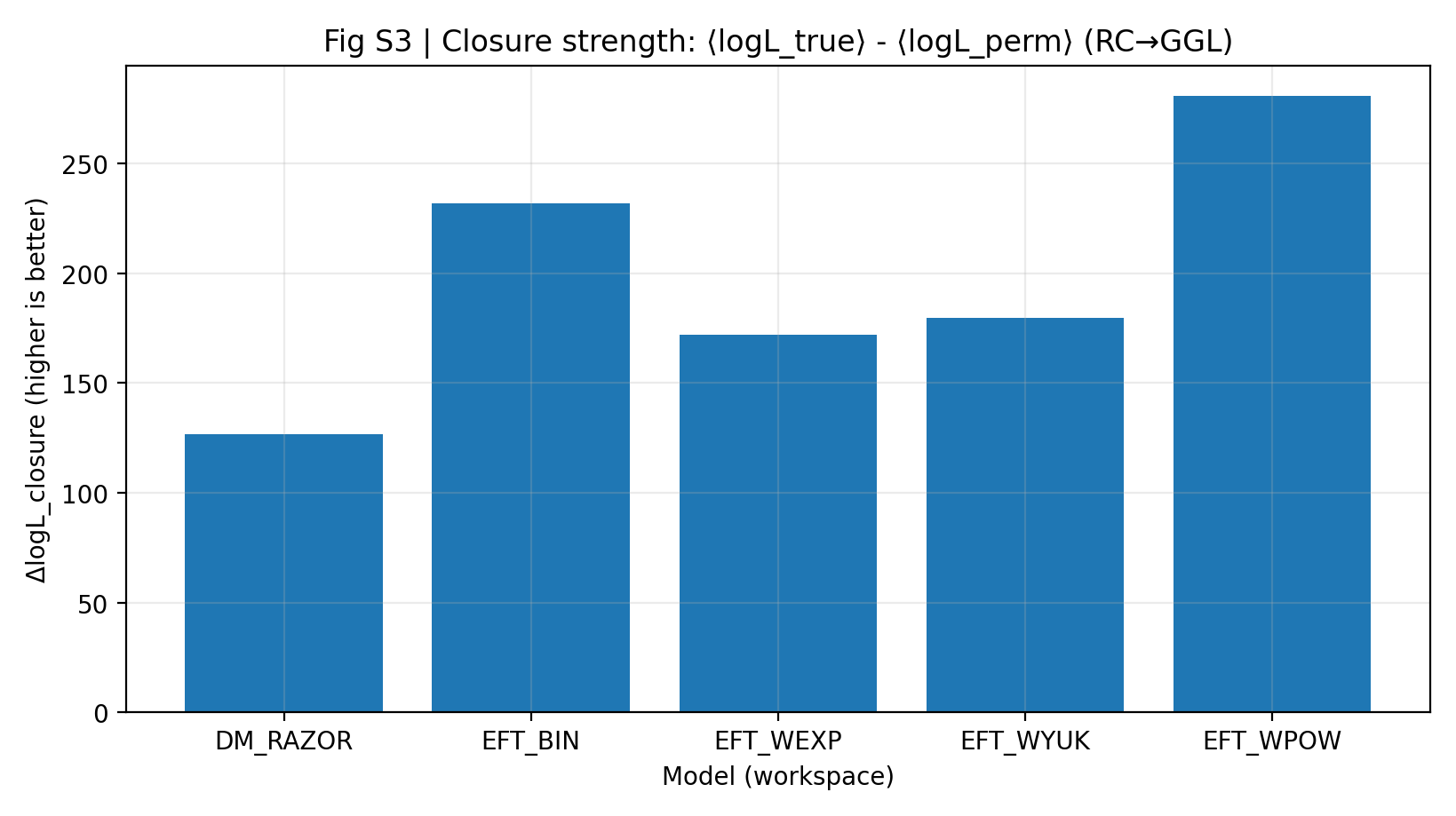
Fig. S3 | Closure strength (higher is better): mean log-likelihood advantage of RC-only → GGL prediction.

2.3 Fig. S4: Main Joint-Fit Comparison (RC+GGL)

The joint-fit advantage is defined as ΔlogL_total ≡ logL_total(model) − logL_total(DM_RAZOR). Under the same data, the same mapping, and nearly the same parameter scale, the EFT family achieves a significantly higher joint log-likelihood.

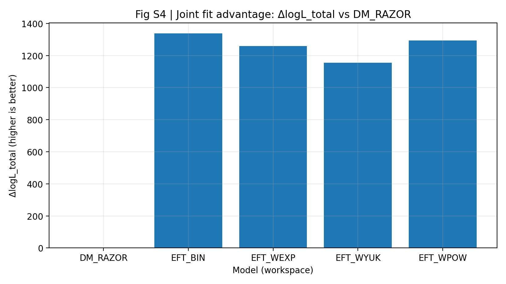
Fig. S4 | Joint-fit advantage (higher is better): best logL_total for RC+GGL relative to DM_RAZOR.

2.4 Four Conclusions (Directly Quotable)

(1) In a unified joint analysis of SPARC rotation curves and KiDS-1000 weak lensing, the EFT mean-gravity framework model systematically outperforms DM_RAZOR under a strict control protocol: ΔlogL_total = 1155–1337 relative to DM_RAZOR.

(2) The RC→GGL closure test shows stronger predictive consistency for EFT: ΔlogL_closure = 172–281, compared with 127 for DM_RAZOR. When the RC-bin→GGL-bin grouping is randomly shuffled, the closure signal collapses to 6–23, indicating that the signal depends on the correct cross-data mapping rather than accidental fitting.

(3) Systematic scans of σ_int, R_min, and covariance shrinkage do not change the sign or scale of “EFT outperforms DM_RAZOR,” indicating that the conclusion is robust to common systematic perturbations.

(4) Under the same closure protocol, Appendix B (P1A) strengthens the DM baseline in a “standardized and auditable” way: it retains three one-parameter enhancements (SCAT/AC/FB) and adds hierarchical c–M scatter + prior, a one-parameter core proxy, and a lensing-side shear-calibration m (and their combined DM_STD model). The results show that only the feedback/core branch brings a small net improvement in closure strength (122.21→129.45, ΔΔlogL_closure≈+7.25); the other enhancements contribute insignificantly or negatively to closure strength. Thus, the main conclusion does not depend on DM_RAZOR being an overly weak baseline.

3 Data and Preprocessing

This study uses two public datasets. Within the engineering workflow, downloading, checksum verification (sha256), and preprocessing are completed with traceable scripts. To ensure fair cross-model comparison, all workspaces (EFT_BIN / EFT_WEXP / EFT_WYUK / EFT_WPOW / DM_RAZOR) share exactly the same data products and bin mappings.

3.1 Rotation Curves (RC, SPARC)

The RC data come from the SPARC database’s Rotmod_LTG files (175 rotmod files). After preprocessing, the modeling sample includes 104 galaxies and 2,295 (r, V_obs) data points, divided into 20 RC bins according to stellar mass and related criteria. Each data point contains radius r (kpc), observed velocity V_obs (km/s), observational error σ_obs, and the gas/disk/bulge component velocities (V_gas, V_disk, V_bul).

3.2 Weak Lensing (GGL, KiDS-1000 / Brouwer+2021)

The GGL data use the excess surface density ΔΣ(R) from Fig. 3 of Brouwer et al. (2021) based on KiDS-1000 (4 stellar-mass bins, 15 R points per bin), together with the provided full covariance. In the engineering workflow, the original long-form covariance is reconstructed into a 15×15 matrix for each bin, and Stage-B audits verify dimensional and numerical reasonableness.

3.3 RC-bin → GGL-bin Mapping and Total Sample Size

The 4 GGL mass bins and 20 RC bins are connected through a fixed mapping: each GGL bin corresponds to 5 RC bins, and RC-bin contributions are weighted by the number of galaxies. This mapping is held fixed across all models and is the core constraint for fair comparison in closure testing and joint fitting. The final joint dataset contains n_total = 2355 points (RC=2295, GGL=60).

4 Models and Statistical Methods

4.1 Minimal Mathematical Specification for EFT and DM (Auditable/Testable)

This section gives the minimal mathematical specification that maps directly to the implementation.

(a) Rotation-curve (RC) model

For each RC data point (r, V_obs, σ_obs), we use component superposition: V_mod²(r) = V_bar²(r) + V_extra²(r). Here V_bar²(r) = V_gas²(r) + Υ_d·V_disk²(r) + Υ_b·V_bul²(r). The main results in this paper adopt Υ_d = Υ_b = 0.5, consistent with SPARC empirical recommendations and useful for reducing unnecessary degrees of freedom.

(b) EFT mean-gravity correction (EFT)

The EFT extra term is parameterized in the form of “mean velocity squared”: V_extra²(r) = V0_bin² · f(r/ℓ). Here V0_bin is the amplitude parameter for each RC bin (20 parameters), ℓ is a global scale (1 parameter), and f(x) is a dimensionless kernel shape function. The kernel shapes compared in this paper (none of which introduce additional continuous degrees of freedom) are:

• none: f(x)=x/(1+x)
• exponential: f(x)=1−exp(−x)
• yukawa: f(x)=1−exp(−x)·(1+0.5x)
• powerlaw_tail: f(x)=1−(1+x)^(−1/2)
• (optional control) gaussian: f(x)=erf(x/√2) (not included in the main conclusion set)

Physical motivation (extended): EFT interprets the extra gravitational response on galaxy scales as an effective response obtained by coarse-graining/scale-averaging more microscopic actions over finite scales. In this paper, we do not assume any specific microscopic mechanism; instead, we use a minimal and auditable parameterization for controlled comparison and testing under a unified statistical protocol.

For intuition, the extra term can be written in acceleration form: a_extra(r)=V_extra²(r)/r=(V0_bin²/r)·f(r/ℓ). When r≫ℓ, f→1 and V_extra→V0_bin, producing an approximately flat outer-region extra velocity contribution. When r≪ℓ and f(x)≈x, a characteristic acceleration scale a0,bin≈V0_bin²/ℓ can be introduced (up to an O(1) kernel-function factor), providing a MOND-like intuition for the inner-to-outer transition scale.

The discrete kernel family used here (none/exponential/yukawa/powerlaw_tail) can be viewed as low-dimensional proxies for different “initial slopes / transition speeds / long-range tails” (for example, Yukawa-like screening versus a longer-tailed response). They are used for robustness stress testing rather than to exhaust the model space. In the weak-lensing component, we construct an effective envelope mass and density from V_avg(r), then project them to obtain ΔΣ(R). This effective density should be understood as an effective description of the lensing potential under the assumptions of spherical symmetry and weak-field mapping (full details are moved to Appendix A).

All of the above kernel shapes satisfy f(x)→1 as x→∞ (i.e., saturation V_extra²→V0²), while giving linear or sublinear growth for x≪1: for example, exponential: f≈x; yukawa: f≈0.5x; powerlaw_tail: f≈0.5x. Therefore, different kernel shapes have observable differences in small-radius “initial slope,” transition speed, and outer tail, and can be distinguished by the joint RC+GGL and closure tests.

The EFT prediction for weak-lensing ΔΣ(R) is obtained by inferring envelope mass and density from V_avg(r), followed by projection integrals: M_enc(r)=r·V_avg²(r)/G, ρ(r)=(1/4πr²)·dM_enc/dr, Σ(R)=2∫_R^∞ ρ(r)·r/√(r²−R²) dr, and ΔΣ(R)=Σ̄(<R)−Σ(R). The numerical implementation uses a logarithmic grid and adaptively refines it in exceptional cases to ensure stability and reproducibility.

(c) DM_RAZOR: NFW cold-dark-matter halo baseline

At the same time, we make clear that DM_RAZOR represents only a minimal, auditable NFW baseline (fixed c–M and no scatter; no adiabatic contraction, feedback core, nonsphericity, or environmental terms). To reduce the risk of a “strawman baseline,” this paper does not claim that such effects do not exist. Instead, it incorporates them in Appendix B (P1A) as low-dimensional and auditable stress tests, including hierarchical treatment of c–M scatter, a core proxy, and a lensing-side shear-calibration nuisance.

4.2 Model Ledger and Fair Comparison (Shared Parameters = Definition of Closure)

The number of parameters in the main comparison set is: DM_RAZOR k=20; EFT family k=21 (the extra parameter is the global log ℓ). All models share the same RC data, the same GGL data and covariance, the same RC-bin→GGL-bin mapping, the same baryonic terms, and the same unit conversions. In addition, the kernel shape (none / exponential / yukawa / powerlaw_tail) is a discrete choice and introduces no additional continuous parameter, preventing an advantage from being gained by “one extra degree of freedom.”

4.3 Likelihood, Priors, and Sampler

The RC likelihood is diagonal Gaussian: σ_eff² = σ_obs² + σ_int². The main results fix σ_int=5 km/s, and Run-5 scans σ_int. The GGL likelihood uses a full-covariance Gaussian for each bin: logL_GGL = Σ_b log 𝒩(ΔΣ_obs^b | ΔΣ_mod^b, C_b). The joint objective is logpost(θ)=logprior(θ)+logL_RC(θ)+logL_GGL(θ). The priors mainly encode physically feasible boundaries (interval constraints on log ℓ, log V0, and log M200); when free Υ and σ_int are enabled, weakly informative priors are used (see the implementation and release-package configuration for details).

The sampler uses an adaptive block Metropolis random walk: each step updates only a random sub-block of the parameter space to improve the acceptance rate in high dimensions, and the step size is lightly adapted by windowed acceptance rate (target acceptance rate about 0.25). The main results use quick mode (settings such as n_steps=800), and each workspace outputs traces, residuals, and PPC plots for manual and scripted audits.

4.4 Closure Test and Negative Control (Definition)

The closure test (Run-2) tests whether the RC-only posterior can predict GGL without refitting GGL. Specifically, it forward-generates ΔΣ(R) for 4 GGL bins from RC-only posterior samples and computes logL_true with the full covariance; it then randomly permutes the RC-bin→GGL-bin group mapping to obtain logL_perm. Closure strength is defined as ΔlogL_closure≡⟨logL_true⟩−⟨logL_perm⟩. In addition, Run-10 randomly regroups the 20 RC bins into 4×5 (shuffle) and recomputes closure, testing how strongly the closure signal depends on the correct mapping.

5 Main Results and Interpretation

5.1 Main Joint-Fit Results (RC+GGL)

The best logL_total from the joint fit and the relative advantage ΔlogL_total (relative to DM_RAZOR) are shown in Table S1a and Fig. S4. In the main comparison set, EFT_BIN has the largest joint advantage (ΔlogL_total=1337.210), while the other EFT kernel shapes also retain significant advantages (1154.827–1294.442). Under information criteria (AICc/BIC), the EFT family also significantly outperforms DM_RAZOR, indicating that the advantage is not due to bias from the number of parameters.

Note: the main contribution to ΔlogL_total≈1337 comes from the RC term (ΔlogL_RC≈1065 in the joint decomposition, about 80%). This can be understood as a modest improvement of about Δχ²≈0.90 per point across N=2295 RC data points, which naturally accumulates to an advantage of order 10^3 under a diagonal Gaussian likelihood. At the same time, GGL and the closure test provide independent cross-dataset constraints, and the ranking remains stable under σ_int, R_min, and cov-shrink stress tests (see Section 6 and Table S1b).

5.2 Closure Test Results (RC-only → GGL)

The key closure-test quantity ΔlogL_closure is reported in Table S1b and Fig. S3. The EFT family has closure strengths of 171.977–280.513, higher than DM_RAZOR’s 126.678. This means that, with no additional cross-data degrees of freedom allowed, the posterior samples obtained by EFT from the RC data have stronger transferable predictive power for the GGL data.

The negative control further supports the physical relevance of the closure signal: when the RC-bin→GGL-bin grouping is randomly shuffled, EFT’s closure strength drops to 6–15 (with small differences among kernels), whereas the baseline closure strength is as high as 172–281. This “signal collapse” rules out false advantages caused by numerical implementation, unit errors, or improper covariance handling.

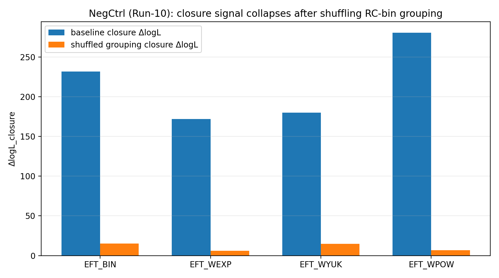
Fig. R1 | Negative control: after shuffle grouping, the closure signal drops significantly (plotted from Tab_Z1 metrics).

5.3 Meaning and Limits of the Results

The conclusion of this study is that “under this dataset and this protocol, the EFT mean-gravity correction outperforms the tested DM_RAZOR baseline.” It must be emphasized that the DM side uses only a minimal NFW baseline with a fixed c(M) relation, without core formation, nonsphericity, environmental terms, or more complex galaxy–halo connection models. Therefore, this manuscript does not claim to exclude all DM model families. Instead, it provides a reproducible, closure-test-centered control baseline for evaluating whether RC and GGL can be consistently explained by the same cross-data parameters and mapping.

To address this common concern, we completed an independent extension project, P1A (see Appendix B). Without changing the RC-bin→GGL-bin shared mapping or audit framework, it strengthens the DM baseline in a “standardized and auditable” manner: beyond three one-parameter enhancements (SCAT/AC/FB), it further adds (i) hierarchical c–M scatter + mass–concentration prior (DM_HIER_CMSCAT), (ii) a one-parameter baryonic-feedback core proxy (DM_CORE1P), and (iii) a weak-lensing-side shear-calibration nuisance m (DM_RAZOR_M), and reports a combined model DM_STD; EFT_BIN is retained as the control reference.

• DM_RAZOR_SCAT (c–M scatter) — introduces the halo-to-halo concentration-scatter parameter σ_logc to test whether a fixed c(M) systematically underestimates DM’s explanatory power;
• DM_RAZOR_AC (Adiabatic Contraction) — uses a single parameter α_AC to continuously interpolate between “no contraction” and “standard contraction,” capturing the tendency of baryons to contract the inner halo at minimal cost;
• DM_RAZOR_FB (Feedback/core) — uses a core scale (e.g., log r_core) to describe how inner-core formation suppresses rotation curves, while maintaining the NFW approximation on weak-lensing scales.

The quantitative P1A scoreboard is provided in Appendix B, Table B1 / Fig. B1 (automatically generated from Tab_S1_P1A_scoreboard). In the closure metric, DM_RAZOR_FB gives a small net improvement (122.21→129.45, +7.25), while the other enhancements contribute insignificantly or negatively to closure strength. On the joint-fit side, adding a hierarchical c–M scatter prior (DM_HIER_CMSCAT) or the combined model (DM_STD) can substantially improve joint logL, but does not improve closure strength, suggesting that it mainly adds joint-fit flexibility rather than cross-probe transferability. Therefore, the core conclusion of the main text should be read as follows: under strict shared-mapping and closure-test constraints, EFT’s cross-data consistency advantage does not arise from choosing an “overly weak baseline” on the DM side. The P1A release package corresponding to Appendix B (supplementary tables/figures and full_fit_runpack) will be included as additional files under the same Zenodo Concept DOI as the full_fit_runpack for this paper: https://doi.org/10.5281/zenodo.18526286.

6 Robustness and Control Experiments

6.1 σ_int Scan (Run-5)

We systematically scan the intrinsic RC scatter σ_int and repeat joint inference at each σ_int, computing ΔlogL_total relative to DM_RAZOR. The minimum/maximum ΔlogL_total values for each model across the scan range are reported in Table S1b.

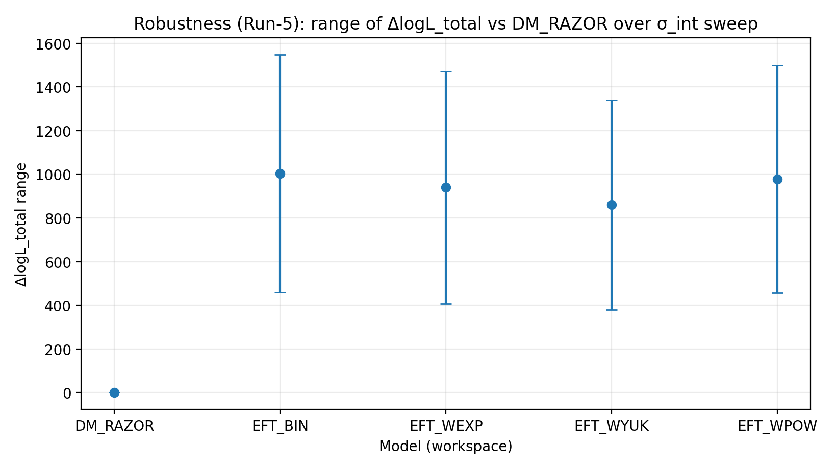
Fig. R2 | Range of ΔlogL_total under the σ_int scan (higher is better).

6.2 R_min Scan (Run-6)

To test the impact of systematics in central-region data (such as noncircular motion, resolution, and insufficient baryonic modeling), we apply R_min threshold cuts to RC and repeat joint inference. The EFT family’s advantage remains positive and stable in scale under the R_min scan.

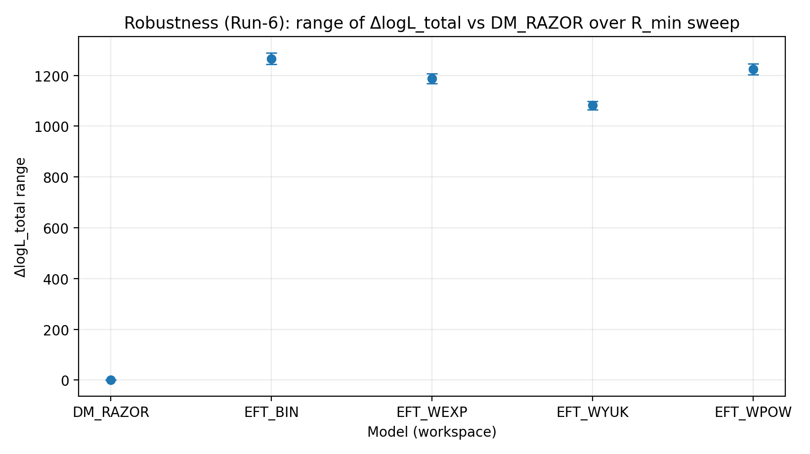
Fig. R3 | Range of ΔlogL_total under the R_min scan (higher is better).

6.3 cov-shrink Scan (Run-7)

To test uncertainty in the GGL covariance, we apply shrinkage to the covariance matrix of each mass bin: C_α=(1−α)C+α·diag(C), and scan α. The results show that the advantage of the EFT family is insensitive to this treatment.

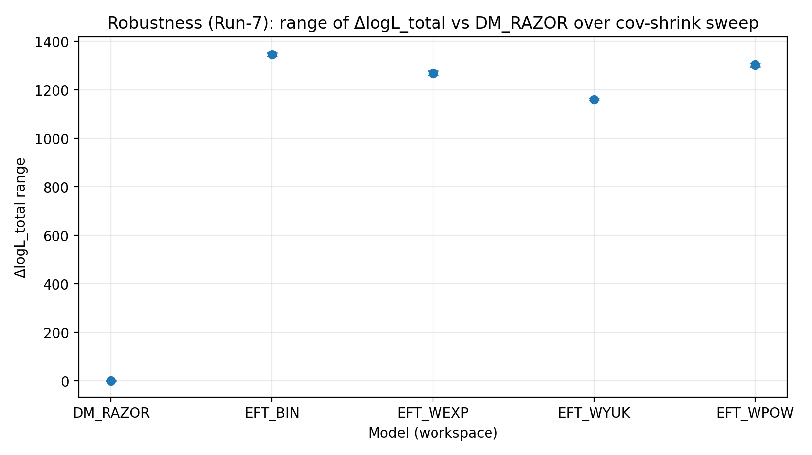
Fig. R4 | Range of ΔlogL_total under the cov-shrink scan (higher is better).

6.4 Ablation Ladder (Run-8)

Within EFT_BIN, we perform nested ablations: from a minimal model (with no free parameters), to versions retaining only a small number of degrees of freedom, and finally to the complete 20-bin amplitude + global scale model. AICc/BIC show that the complete EFT_BIN model is strongly required by the data.

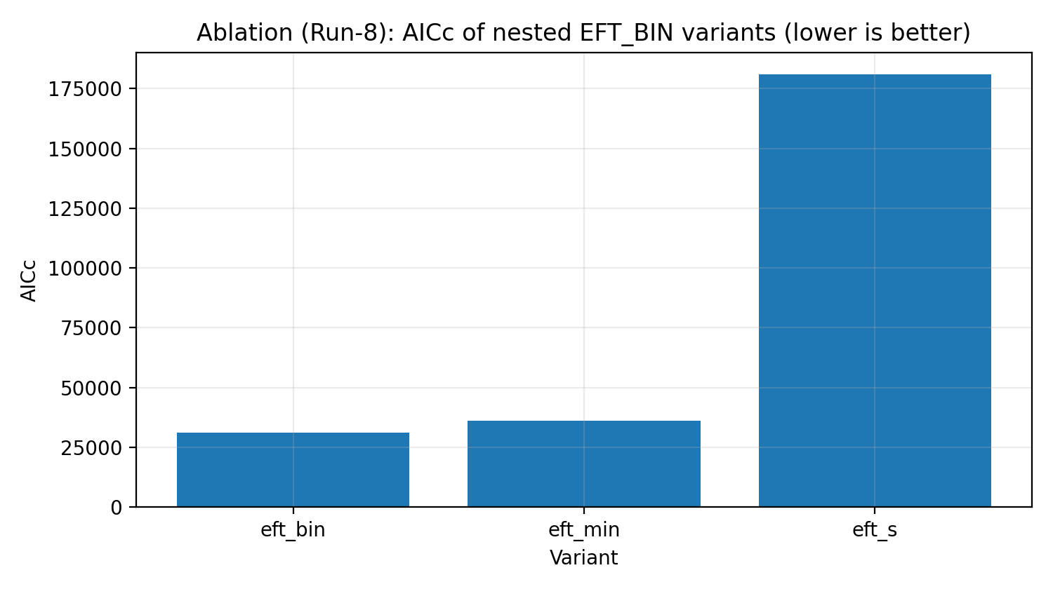
Fig. R5 | EFT_BIN ablation ladder (AICc; lower is better).

6.5 Holdout Prediction (Run-9)

We further run a leave-one-bin-out (LOO) test: among the 4 GGL mass bins, one bin is held out each time; inference is redone using the remaining bins (and all RC), and the test log-likelihood is then evaluated on the held-out bin. Summary metrics are given in the supplementary table Tab_R3_leave_one_bin_out (a Run-9 product; file path patterns are listed in the key-product list in Section 8.2). The EFT family remains clearly superior to DM_RAZOR even in the worst held-out case.

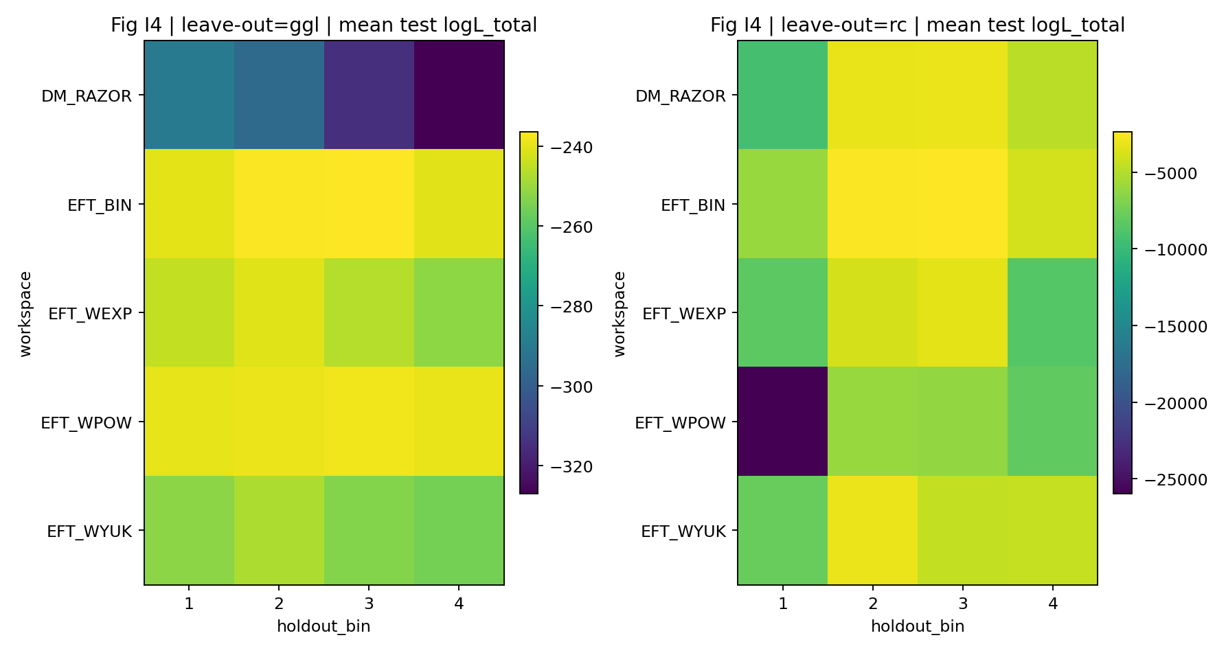
Fig. R6 | LOO: log-likelihood distribution for the held-out bin (from Run-9 products).

6.6 Negative Control: RC-bin Shuffle (Run-10)

Run-10 randomly regroups the 20 RC bins into 4×5 and recomputes closure while keeping the RC-only posterior unchanged. The results show that, compared with the original mapping, shuffling significantly lowers both the closure mean logL_true and ΔlogL_closure (see Table S1b and Fig. R1), further supporting the interpretability of the closure signal.

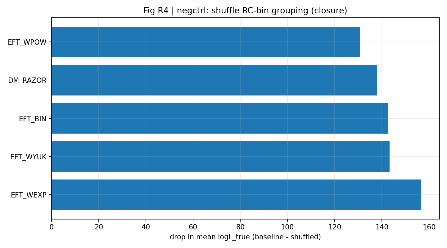
Fig. R7 | Negative control: shuffle mapping causes a clear drop in closure mean logL_true (from Run-10 products).

7 Traceability and Consistency Audit (Provenance)

All numerical values cited in this paper can be traced item by item in the strict summary tables and audit records of the release archive. To keep the main text more readable, the full provenance chain (tag list, audit tables, checksum list, and verification method) has been moved to Appendix A.

8 Reproducibility and Zenodo Archive

Data and code availability statement: the SPARC rotation-curve data and KiDS-1000 weak-lensing data used in this paper are public datasets. The publication-grade report has been archived on Zenodo (Concept DOI: https://doi.org/10.5281/zenodo.18526334), and the full reproduction package has been archived on Zenodo (Concept DOI: https://doi.org/10.5281/zenodo.18526286). Detailed execution steps, dependency environment, archive inventory, and hash-verification information are provided in Appendix A; the design, run tags, and outputs of the DM-baseline standardization stress test (P1A) are provided in Appendix B.

Under the same full-reproduction-package Concept DOI (https://doi.org/10.5281/zenodo.18526286), we provide two reproducible entry points by use case: • P1 (main text) full_fit_runpack: reproduces the RC-only / closure / joint analyses and robustness scans for EFT vs DM_RAZOR, and generates main-text assets including Tables S1a/S1b and Figs. S3/S4; • P1A (Appendix B) full_fit_runpack: reproduces the DM-baseline standardization stress test (SCAT/AC/FB + hierarchical c–M scatter prior + core1p + lensing m + DM_STD, including the EFT_BIN control), and generates Appendix Table B1 and Fig. B1. P1A’s supplementary tables/figures and full_fit_runpack will be included as additional files under the same Concept DOI to maintain a single archive entry point.

9 Acknowledgments and Declarations

9.1 Acknowledgments

We thank the SPARC and KiDS-1000 teams for providing public data and documentation, and the participants in this project’s reconstruction and audit workflow.

9.2 Author Contributions

Guanglin Tu was responsible for the conceptual proposal, study design, engineering implementation, data curation, formal analysis, reproducibility workflow implementation and audit, and manuscript writing.

9.3 Funding

Self-funded by the author, Guanglin Tu (no external funding / no grant number).

9.4 Competing Interests

The author, Guanglin Tu, is affiliated with the “EFT Working Group, Shenzhen Energy Filament Science Research Co., Ltd. (China)”; no other competing interests are declared.

9.5 AI Assistance

OpenAI GPT-5.2 Pro and Gemini 3 Pro were used for language polishing, structural editing, and organization of the reproducibility workflow. They were not used to generate or modify data, results, figures, tables, or code, nor to generate citations. The author bears full responsibility for the content and citation accuracy of the entire manuscript.

10 References

• Lelli, F., McGaugh, S. S., & Schombert, J. M. (2016). SPARC: Mass Models for 175 Disk Galaxies with Spitzer Photometry and Accurate Rotation Curves. The Astronomical Journal, 152, 157. DOI: 10.3847/0004-6256/152/6/157.
• Brouwer, M. M., Oman, K. A., Valentijn, E. A., et al. (2021). The weak lensing radial acceleration relation: Constraining modified gravity and cold dark matter theories with KiDS-1000. Astronomy & Astrophysics, 650, A113. DOI: 10.1051/0004-6361/202040108.
• Wright, C. O., & Brainerd, T. G. (2000). Gravitational Lensing by Navarro–Frenk–White Halos. The Astrophysical Journal, 534, 34–40.
• Navarro, J. F., Frenk, C. S., & White, S. D. M. (1997). A Universal Density Profile from Hierarchical Clustering. Astrophysical Journal, 490, 493. DOI: https://doi.org/10.1086/304888
• Dutton, A. A., & Macciò, A. V. (2014). Cold dark matter haloes in the Planck era: evolution of structural parameters for NFW haloes. Monthly Notices of the Royal Astronomical Society, 441, 3359–3374. DOI: https://doi.org/10.1093/mnras/stu742
• Blumenthal, G. R., Faber, S. M., Flores, R., & Primack, J. R. (1986). Contraction of dark matter galactic halos due to baryonic infall. Astrophysical Journal, 301, 27. DOI: https://doi.org/10.1086/163867
• Di Cintio, A., Brook, C. B., Dutton, A. A., et al. (2014). A mass-dependent density profile for dark matter haloes including the influence of galaxy formation. Monthly Notices of the Royal Astronomical Society, 441, 2986–2995. DOI: https://doi.org/10.1093/mnras/stu729
• Read, J. I., Agertz, O., & Collins, M. L. M. (2016). Dark matter cores all the way down. Monthly Notices of the Royal Astronomical Society, 459, 2573–2590. DOI: https://doi.org/10.1093/mnras/stw713
• Energy Filament Theory. Zenodo (open science repository) DOI: https://doi.org/10.5281/zenodo.18517411

Appendix A: Traceability and Reproducibility Details

This appendix summarizes long-term archive information for traceability and reproducibility, including run tags, audit results, archive inventories, and key verification points, so that readers can check and reproduce the work as needed.

A.1 Traceability and Audit Details

To ensure long-term traceability, this project uses timestamped tags for each run and output, and keeps historical products without overwriting them. The core values cited in this manuscript come from the strict compilation (compile_tag=20260205_035929) and have passed the following consistency audits:

• All stage-level tables carry run_tag and stage tags; the strict compilation script selects “complete and consistent” canonical table sources from report/tables.

• Values in Tab_Z1_master_summary and Tab_Z2_conclusion_highlights are compared item by item against the selected canonical tables.

• During PDF generation, a tag audit is performed on “referenced table/figure tags” to ensure that outdated products are not mixed in.

Key tags (for locating all intermediate products): run_tag=20260204_122515; closure_tag=20260204_124721; joint_tag=20260204_152714; sigma_sweep_tag=20260204_161852; rmin_sweep_tag=20260204_195247; covshrink_tag=20260204_203219; ablation_tag=20260204_214642; LOO_tag=20260204_224827; negctrl_tag=20260204_234528; strict_compile_tag=20260205_035929; release_tag=20260205_112442.

Consistency-audit result: Tab_AUDIT_checks_strict reports pass=9, fail=0, skip=0 (see the release package for details).

A.2 Reproducibility Execution Steps and Archive Inventory

This study adopts a reproducibility system consisting of “publication-grade report + tables/figures supplement + fully rerunnable run package.” Readers can directly consult the Tables & Figures Supplement to verify all table/figure assets cited in the paper; to reproduce numerical values and the audit chain from scratch, they can use the full_fit_runpack to download the data and rerun the complete workflow. After completion, the package’s built-in reference-table comparison script can be used to verify table-value consistency.

A.2.1 Reproduction Quickstart (RUN_FULL, Windows PowerShell)

This section gives a shorter reproduction path (Windows PowerShell). For quick checks, readers are advised to consult the Tables & Figures Supplement directly and verify the cited tables and figures item by item. For end-to-end reproduction and generation of all tables, figures, and audit products, use the full_fit_runpack: follow the package README/ONE_PAGE_REPRO_CHECKLIST to run verify_checksums.ps1 and RUN_FULL.ps1 (Mode=full recommended).

Zenodo archive entry (Concept DOI): https://doi.org/10.5281/zenodo.18526286.
Main-chain tags for this paper: run_tag=20260204_122515; strict compile_tag=20260205_035929; release_tag=20260205_112442.

A.2.2 Archive Materials and Key Verification Points (Packages & checks)

The Zenodo archive provides three complementary categories of materials: (1) publication-grade report (this paper, v1.1; including Appendix B: P1A DM-baseline standardization stress test); (2) Tables & Figures Supplement (supplementary tables and figures covering all table/figure assets cited in this paper, corresponding separately to P1 and P1A); and (3) full_fit_runpack (full reproduction package: downloads data from scratch and reruns the complete workflow, corresponding separately to P1 and P1A). Items (1)–(2) support quick reading and independent verification; item (3) provides end-to-end full reproducibility.

Citation recommendation: when citing this paper or the accompanying reproducibility materials, please cite the Zenodo Concept DOI (https://doi.org/10.5281/zenodo.18526334).

Key products that should appear and be comparable after reproduction include:

• report/tables/Tab_D_closure_summary__20260204_122515__*.csv (closure summary)
• report/tables/Tab_F_joint_summary__20260204_122515__*.csv (joint-fit summary)
• report/tables/Tab_G_joint_sigma_sweep__20260204_122515__*.csv (σ_int scan)
• report/tables/Tab_H_joint_rmin_sweep__20260204_122515__*.csv (R_min scan)
• report/tables/Tab_I_joint_covshrink_sweep__20260204_122515__*.csv (cov-shrink scan)
• report/tables/Tab_R2_ablation_ladder__20260204_122515__*.csv (ablation)
• report/tables/Tab_R3_leave_one_bin_out__20260204_122515__*.csv (LOO)
• report/tables/Tab_R4_negctrl_rcbin_shuffle__20260204_122515__*.csv (negative control)
• report/final/Tab_Z1_master_summary__20260204_122515__20260205_035929.csv (Strict master table; corresponds to Tables S1a/S1b and main-text values)
• report/final/P1_RC_GGL_final_bundle__20260204_122515__20260205_035929.pdf (publication-grade PDF bundle; can be used for quick browsing and citation)

Appendix B: P1A—DM-Baseline Standardization Stress Test (DM 7+1 + DM_STD; with EFT Control)

This appendix documents an extension project (P1A) for “DM-baseline standardization stress testing” that is consistent with the closure protocol in the main text. Its role is to upgrade the minimal DM_RAZOR baseline used in the main text (NFW + fixed c–M, no scatter / no contraction / no core) into a DM baseline set that is closer to astrophysical practice and more resistant to common critiques, without introducing a large number of degrees of freedom and without changing the RC-bin→GGL-bin shared mapping or audit framework. P1A covers, and is a superset of, the earlier three-branch stress test: it retains SCAT/AC/FB while adding hierarchical c–M scatter + prior, a one-parameter core proxy, and a lensing-side shear-calibration nuisance m; it also provides the combined model DM_STD. EFT_BIN is retained as the control reference.

Supplementary note: closure strengths and related values in Appendix B (P1A) use a larger Monte Carlo budget (for example, ndraw=400, nperm=24) than the quick budget used in the main text to cover the full EFT kernel family (for example, ndraw=60, nperm=12). Therefore, absolute values may show O(10)-level sampling drift. However, model-to-model comparisons within the same budget/table are fair, and the sign and scale of the advantage remain stable across budgets.

B.1 Purpose and Positioning (Why P1A, and Why as an Appendix)

P1A does not attempt to exhaust all possible ΛCDM halo modeling choices (such as nonsphericity, environmental dependence, complex galaxy–halo connections, or high-dimensional baryon physics). Instead, P1A follows a “low-dimensional, auditable, reproducible” principle: each enhancement module introduces only ≤1 key effective parameter and remains subject to the three hard constraints of this paper:
(i) Parameter ledger: every new parameter must be explicitly recorded and reported together with information criteria (AICc/BIC);
(ii) Shared mapping: the same RC-bin→GGL-bin grouping map is still used; “tuning the mapping” separately for a single dataset is not allowed;
(iii) Closure test: any enhancement must show genuine gain in RC→GGL transfer prediction, not merely better RC-only fitting.

B.2 DM 7+1 + DM_STD: Module Definitions, Parameters, and Entry into the Joint Posterior

As an independent runpack, P1A provides 8 DM workspaces (DM 7+1) plus 1 EFT control: starting from DM_RAZOR as the baseline, it constructs three legacy one-parameter enhancements (DM_RAZOR_SCAT / DM_RAZOR_AC / DM_RAZOR_FB), adds three more standard defensive modules (DM_HIER_CMSCAT / DM_CORE1P / DM_RAZOR_M), and then provides the combined model DM_STD. The shared goal of these modules is to cover the three most common critiques while increasing dimensionality as little as possible: (a) how c–M scatter and priors enter a hierarchical model; (b) whether the main effect of baryonic feedback can be captured by a one-parameter core proxy; and (c) whether key lensing-side systematics could be mistaken for a physical signal.

Note: the parameter names above follow the engineering implementation (for example, σ_logc, α_AC, log r_core, and m_shear). The design focus of P1A is to “make the DM baseline somewhat stronger while keeping it auditable,” not to turn the DM side into an uncontrollable high-dimensional fitter. In particular, DM_HIER_CMSCAT introduces c–M scatter hierarchically: the concentration c_i of each halo is assigned a log-normal scatter around c(M_i), constrained by the global σ_logc and the c(M) prior; this hierarchical structure affects the joint posterior of both RC and GGL.

B.3 Statistical Protocol and Product Conventions Consistent with the Main Text

P1A reuses all data products, the shared mapping, and the audit framework from the main text. The execution order and product conventions remain consistent:
(1) Run‑1: RC-only inference (outputs posterior_samples.npz and metrics.json);
(2) Run‑2: RC→GGL closure test (outputs closure_summary.json and the permuted baseline);
(3) Run‑3: RC+GGL joint fit (outputs joint_summary.json).
All quoted numbers come from the automatically compiled table (Tab_S1_P1A_scoreboard) and can be checked after rerunning the full P1A workflow using the reference-table comparison script built into the P1A full_fit_runpack.

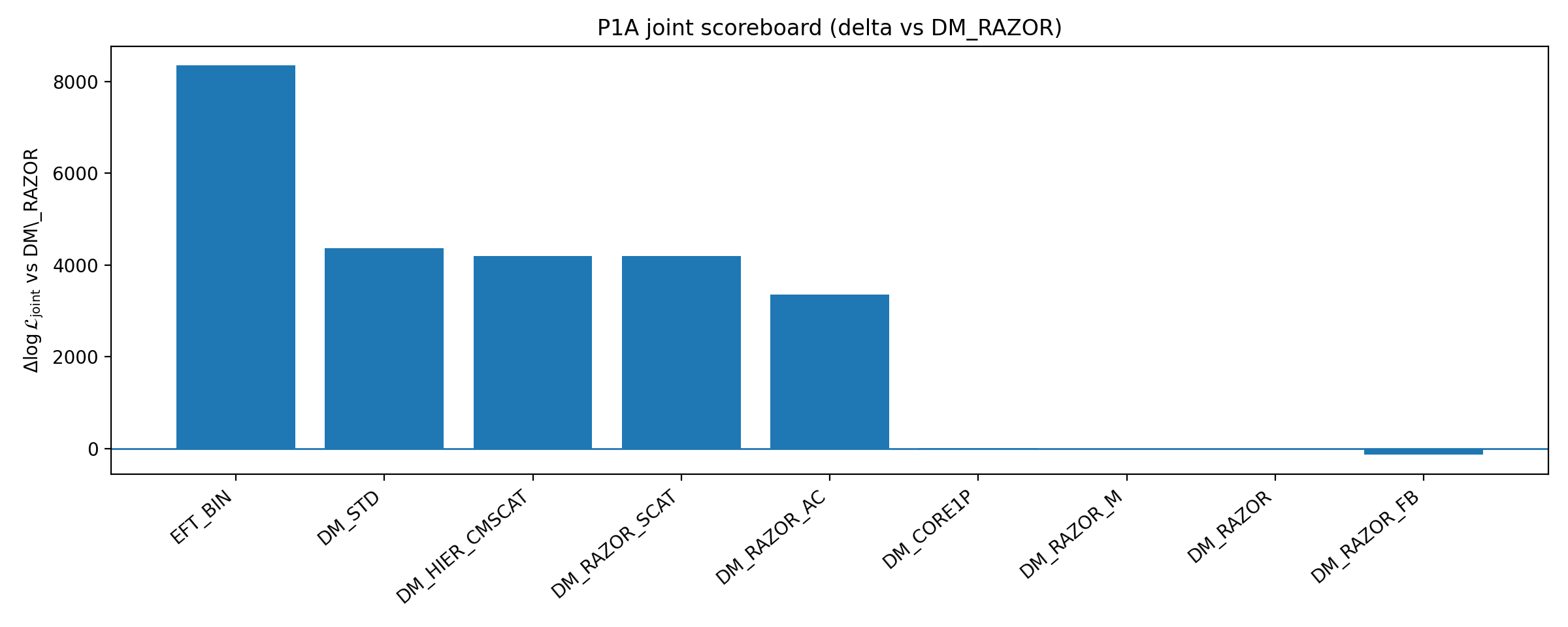
B.4 Main Results, Table/Figure Entry Points, and Archive Plan (Same DOI)

This section gives the core quantitative conclusions of P1A. Table B1 summarizes key metrics for RC-only, RC→GGL closure, and RC+GGL joint fitting (parentheses give differences relative to the DM_RAZOR baseline). Closure strength is defined as ΔlogL_closure ≡ ⟨logL_true⟩ − ⟨logL_perm⟩ (higher is better). Fig. B1 visualizes the same scoreboard. The main points are as follows:
• Among the three legacy branches, only DM_RAZOR_FB (feedback/core) gives a small net improvement in closure strength: 122.21→129.45 (+7.25); SCAT and AC provide no net improvement;
• The newly added DM_HIER_CMSCAT and DM_RAZOR_M have very small effects (~0) on closure strength, and DM_CORE1P likewise shows no significant net improvement;
• The combined model DM_STD can substantially improve joint logL (closer to the joint-fit optimum), but its closure strength decreases, suggesting that its gain mainly comes from joint-fit flexibility rather than cross-probe transferability;
• As a control, EFT_BIN still retains a clear advantage in both closure strength and joint fitting. Therefore, the main conclusion is robust to the introduction of a “stronger DM baseline + lensing nuisance.”

For direct comparison with the main-text results, Tables S1a–S1b summarize the strict comparison between the EFT family and DM_RAZOR: EFT models improve the joint fit by ΔlogL_total≈1155–1337 relative to DM_RAZOR and reach ΔlogL_closure=172–281 in the closure test. P1A only creates a “harder control” on the DM side; its purpose is to reduce concerns such as “strawman baseline” or “systematics-as-physics,” not to replace the main comparison.

Table B1 | P1A scoreboard (higher is better; parentheses indicate differences relative to the DM_RAZOR baseline).

Fig. B1 | P1A scoreboard: closure and joint ΔlogL relative to baseline (higher is better).

Example tags for the completed run set corresponding to this appendix are as follows (used to locate P1A intermediate products and tables/figures):
P1A run_tag = 20260213_151233; P1A closure_tag = 20260213_161731; P1A joint_tag = 20260213_195428.

B.5 Suggested Citation (Appendix Citation Note)

When readers need to cite the “DM-baseline standardization stress test” in addition to the main conclusions of the paper, it is recommended that they cite the main conclusion together with the following note: “See Appendix B (P1A) for standardized DM-baseline stress tests (legacy SCAT/AC/FB + hierarchical c–M scatter prior + core proxy + lensing shear-calibration nuisance), under the same closure protocol.”