P1 Report Explained — From Rotation Curves to Weak Lensing: Testing EFT’s Mean Gravitational Response
A public-facing guide based on P1_RC_GGL: A Strict Closure Test of Galaxy Dynamics and Weak Lensing (v1.1)
Check the original evaluation report:
1. ChatGPT: https://chatgpt.com/share/6a00cd62-6e34-83eb-b165-6ec09e3519cc
2. Gemini: https://gemini.google.com/share/773ec96d75a0
3. Grok: https://grok.com/share/bGVnYWN5LWNvcHk_c0b4fa65-0e86-4adb-9b58-5617d616dc04
4. Qwen: https://chat.qwen.ai/s/22ab9336-671f-420a-a7fa-43e24774bb2a?fev=0.2.46
5. DeepSeek: https://chat.deepseek.com/share/tj6k7hb5owtoldg2bm
Reading Note |
This is an explanatory version, not a separate academic report. It is based on the original P1 report, keeps the key figures and tables, and adds plain-language explanations of what each major step means. |
This guide explains only what P1 concludes under its specified datasets, parameter ledger, and statistical protocol: in the joint test of galaxy rotation curves (RC) and galaxy–galaxy weak lensing (GGL), EFT’s mean gravitational response model clearly outperforms the minimal DM_RAZOR baseline tested here. |
This guide does not interpret P1 as a claim that “dark matter has been overturned.” P1 is only the first step in the P-series experiments. It tests one observable layer of EFT—the “mean gravity floor”—not the full content of the complete EFT framework. |
0 | Understanding P1 in Five Minutes: What Is This Test Doing?
Think of P1 as a cross-probe consistency test. It does not merely ask whether a model can fit one dataset. Instead, it puts two very different gravitational readouts on the same audit bench: rotation curves (RC) read the dynamics inside galaxy disks, while galaxy–galaxy weak lensing (GGL) reads the projected gravitational response on larger scales.
- RC is like a speedometer: it tells us how fast gas and stars rotate at different radii in a galaxy disk.
- GGL is like a scale: by measuring how foreground galaxies slightly bend the light from background galaxies, it infers the average gravitational/mass distribution around galaxies on larger scales.
- P1’s central question is this: can the same model learn a pattern from RC first, then transfer that pattern to GGL and still make sense?
P1 in One Sentence |
P1 raises the bar from “does it fit one probe well?” to “does it close across probes?” A model is more likely to have captured a gravitational structure shared by RC and GGL only if it performs well under the correct mapping and the signal collapses after the mapping is shuffled. |
Table 0 | P1’s Core Numbers and How to Read Them
Metric | Reading in P1 / P1A | Plain-Language Meaning |
Joint-fit ΔlogL_total | In the main-text comparison, EFT is 1155–1337 above DM_RAZOR | The total score difference across the two datasets; larger means a better overall explanation. |
Closure strength ΔlogL_closure | In the main-text comparison, EFT is 172–281, while DM_RAZOR is 127 | The ability to predict GGL after inference from RC alone; larger means stronger cross-probe self-consistency. |
Negative-control shuffle | After shuffling RC-bin→GGL-bin, the EFT closure signal falls to 6–23 | If the correct correspondence is broken, the advantage should disappear; the sharper the collapse, the better it rules out a spurious signal. |
P1A multi-DM stress test | DM 7+1 + DM_STD, with EFT_BIN retained as a comparison | P1A does not look only at the minimal DM_RAZOR baseline. It places multiple low-dimensional, auditable DM enhancement branches into the same closure protocol. |
1 | Why Do P1? Where Is Galaxy-Scale Cosmology Stuck?
Galaxy-scale problems have remained hard because the “extra gravity/mass requirement” is not just a rotation-curve phenomenon. Many observations show a tight connection between visible baryonic matter in galaxies and the actual dynamical/lensing readouts. For the dark-matter route, this means that dark halos, baryonic feedback, galaxy formation history, and observational systematics must be coordinated with great precision. For non-dark-matter gravity routes, it means a model cannot merely look good on RC; it must also survive weak lensing, population scaling relations, and negative controls.
That is the motivation for P1. It does not begin from “dark matter is wrong” or “EFT must be right.” It takes one testable claim into audit: can EFT’s mean gravitational response leave a reproducible, transferable signal in RC→GGL cross-probe closure?
External Literature Context: Why the RC+GGL Window Matters |
The radial acceleration relation (RAR) proposed by McGaugh, Lelli, and Schombert in 2016 shows a tight, low-scatter correlation between the observed acceleration traced by rotation curves and the acceleration predicted from baryonic matter. This makes “baryon–gravity-response coupling” unavoidable for galaxy-scale theory. |
Brouwer et al. (2021) used KiDS-1000 weak lensing to extend the RAR to lower accelerations and larger radii, comparing MOND, Verlinde emergent gravity, and LambdaCDM models. They also noted that differences between early- and late-type galaxies, gas halos, and the galaxy–halo connection remain key explanatory issues. |
Mistele et al. (2024) further used weak lensing to infer circular-velocity curves for isolated galaxies, reporting no clear decline out to several hundred kpc and even to roughly 1 Mpc, in agreement with the BTFR. This shows that weak lensing is becoming an important external readout for testing galaxy-scale gravitational response. |
Therefore, P1’s value is not that it is the “first to discuss RC and GGL together.” Its value is that it places them inside an auditable protocol built from a fixed mapping, a parameter ledger, RC-only→GGL closure, shuffle negative controls, and P1A multi-DM stress tests.
2 | What Does EFT Mean in P1? It Is Not Effective Field Theory
Here, EFT refers to Energy Filament Theory (EFT), not the Effective Field Theory commonly used in physics. In the P1 technical report, EFT is used with restraint: it does not enter the comparison as a complete final theory, but is first compressed into an observable, fit-ready, falsifiable parameterization of “mean gravitational response.”
In plain language, P1 does not start by discussing every microscopic source of extra gravity, and it does not try to prove the whole EFT framework at once. It asks a narrower and harder question: if some mean extra gravitational response exists on galaxy scales, can it first explain RC and then transfer to predict GGL?
Which Part of EFT Does P1 Test? |
P1 targets the “mean gravity floor”: a statistically stable mean contribution that can transfer across samples. |
P1 does not yet handle the “stochastic/noise floor”: the random terms, individual differences, or additional scatter that more microscopic fluctuation processes might introduce. |
P1 also does not address the complete microscopic mechanism, abundance, lifetime, or global cosmological constraints. It is the first step in the P-series experiments, not a final verdict. |
3 | The P1 Series Plan: Why Start with the “Mean Floor”?
The P series can be understood as EFT’s observational retrieval program. It does not lay out every claim at once; instead, it isolates the part most readily testable with public data. P1’s strategy is to test the mean term first: if mean gravitational response cannot even close from RC to GGL, then discussing more complex noise terms or microscopic mechanisms lacks a proper entry point.
Table 1 | Layered Positioning of the P Series
Layer | Question Asked | Role in P1 |
P1 | Can mean gravitational response close in RC→GGL? | Main question of the present report |
P1A | If the DM side is strengthened, does the conclusion remain stable? | Appendix B: DM 7+1 + DM_STD stress test |
Later P-series work | Can the protocol be extended to more data, more probes, and more complex systematics? | Direction for future work |
Deeper-level questions | How do the mean term, noise term, and microscopic mechanism connect? | Outside P1’s conclusion scope |
4 | What Are the Data? What Do RC and GGL Tell Us?
4.1 Rotation Curves (RC): The “Speed Gauge” Inside Galaxy Disks
Rotation curves record how fast gas and stars orbit the center of a galaxy at different radii. The faster the rotation, the stronger the required centripetal force at that radius—and therefore the stronger the effective gravity. P1 uses the SPARC database, with preprocessing that includes 104 galaxies and 2,295 velocity data points, divided into 20 RC-bins.
4.2 Weak Lensing (GGL): A Larger-Scale “Gravity Scale”
Galaxy–galaxy weak lensing measures how foreground galaxies slightly bend the light from background galaxies. It corresponds to projected gravitational response on larger, halo-scale radii and does not depend on the details of gas dynamics inside a galaxy. P1 uses the public GGL data from KiDS-1000 / Brouwer et al. (2021): 4 stellar-mass bins, 15 radial points per bin, 60 data points in total, with the full covariance used.
4.3 Fixed Mapping: Why 20 RC-bins → 4 GGL-bins Matters
P1 connects the 20 RC-bins to the 4 GGL-bins through a fixed rule: each GGL-bin corresponds to 5 RC-bins, combined by galaxy-count-weighted averaging. This mapping is kept unchanged for all models and acts as a hard constraint for closure testing and fair comparison.
Why Not Tune the Mapping Afterward? |
If one could choose after the fact “which RC-bins correspond to which GGL-bins,” a model might manufacture closure by rearranging the correspondence. P1 locks the 20→4 mapping in advance and deliberately breaks it with a shuffle negative control precisely to judge whether the closure signal truly depends on a physically reasonable correspondence. |
5 | Models and Methods: What Exactly Is P1 Comparing?
5.1 The EFT Side: Low-Dimensional Mean Gravitational Response
On the EFT side, a low-dimensional extra-velocity term is used to describe mean gravitational response. The shape of the extra term is controlled by a dimensionless kernel function f(r/ℓ), where ℓ is the global scale, and the amplitude is assigned by RC-bin. Different kernels represent different initial slopes, transition speeds, and long-range tails, and are used for robustness stress tests.
5.2 The DM Side: The Main-Text Comparison and Appendix P1A Must Be Read Separately
In the main-text comparison, DM_RAZOR is a minimized, auditable NFW baseline: it uses a fixed c–M relation and does not include halo-to-halo scatter, adiabatic contraction, feedback cores, non-sphericity, or environmental terms. The strength of this design is controlled degrees of freedom and easy reproducibility; its weakness is that it cannot represent every LambdaCDM or dark-matter-halo model.
Therefore, in Appendix B (P1A), the DM side is turned into a set of “standardized stress tests.” Without changing the shared mapping or closure protocol, P1A gradually adds low-dimensional enhancement branches such as SCAT, AC, FB, HIER_CMSCAT, CORE1P, lensing m, and the combined baseline DM_STD, while retaining EFT_BIN as a comparison. In short, P1A is not a comparison against only one minimal DM baseline; it measures a set of common, auditable DM mechanisms with the same “closure ruler.”
The Precise Conclusion Framing Used Here |
Main text: the EFT family substantially outperforms the minimal DM_RAZOR in the main comparison. |
Appendix B / P1A: under multiple low-dimensional, auditable DM enhancement branches and the DM_STD stress test, some DM joint fits improve, but closure strength does not eliminate EFT_BIN’s advantage. |
The safest statement is therefore: within P1/P1A’s data, mapping, parameter ledger, and closure protocol, EFT mean gravitational response shows stronger cross-data consistency; this is not the same as excluding all dark-matter models. |
5.3 Closure Testing: P1’s Most Important Experimental Syntax
1. Fit using RC alone to obtain a set of RC-only posterior samples.
2. Do not retune with GGL; use the RC posterior directly to predict GGL.
3. Use the full covariance to compute the GGL prediction score under the correct mapping, logL_true.
4. Randomly permute the RC-bin→GGL-bin correspondence to compute the negative-control score, logL_perm.
5. Subtract the two to obtain closure strength: ΔlogL_closure = <logL_true> − <logL_perm>.
Plain-Language Analogy |
A closure test is like a cross-exam retest. The model first learns patterns in the RC exam room, then answers in the GGL exam room. If it has learned a shared rule rather than a local trick, it should still answer well after switching rooms; if the correspondence between exam rooms is deliberately shuffled, the advantage should disappear. |
5.4 Before Reading the Technical Tables: Four Entry Points
Table 5.4 | Reading Path for the Next Set of Landscape Technical Tables
Entry Point | What to Look At | Why It Matters |
Table S1a | RC+GGL joint-fit total score | Answers: “When the two datasets are viewed together, whose overall explanation is stronger?” |
Table S1b | Closure strength, shuffle, and robustness scans | Answers: “Can what was learned from RC transfer to GGL?” |
Table B0 | Definitions of multiple DM enhancement branches in P1A | Prevents P1 from being reduced to “only a comparison with minimal DM_RAZOR.” |
Table B1 | P1A closure and joint-fit scoreboard | Checks whether the closure advantage disappears after DM is strengthened. |
Layout Note |
Landscape pages begin on the next page so the wide tables from the original report can be kept intact without deleting columns or compressing them into unreadability. The body text has already given a plain-language reading; the landscape technical tables are for readers who need to verify values and model branches. |
Figure 0.1 | P1’s Closure-Test Workflow in One Diagram
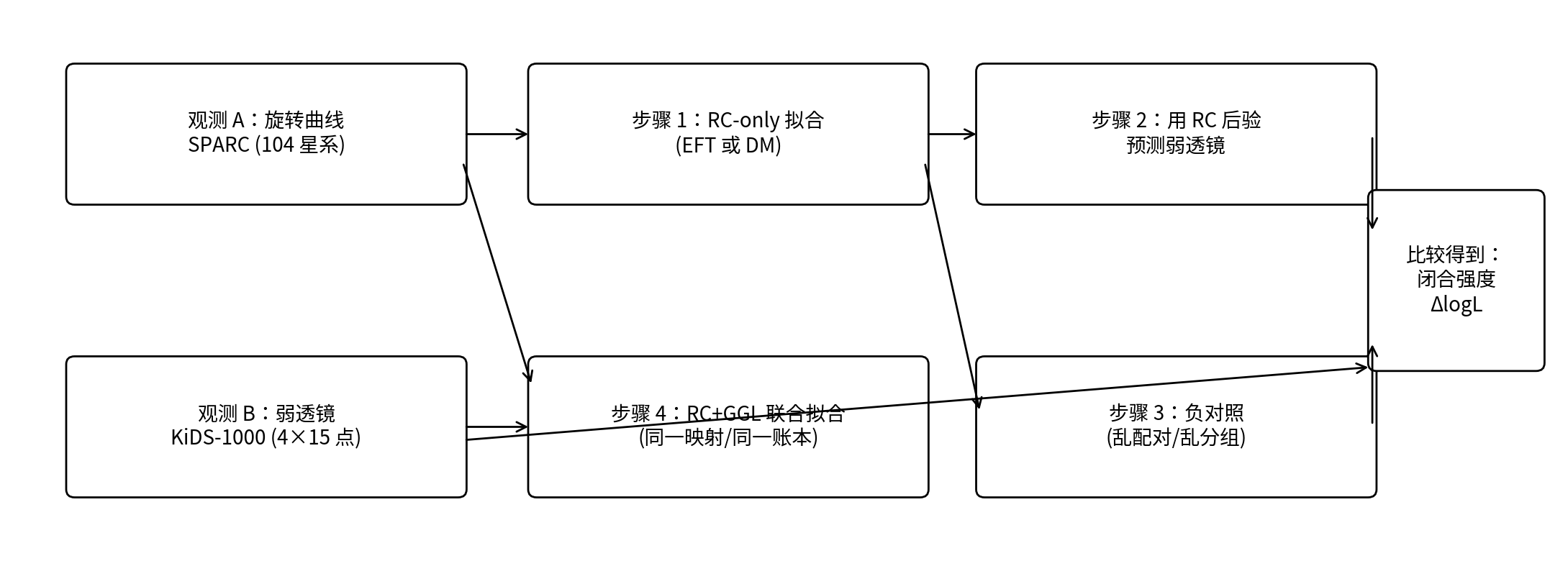
Note: the upper chain is the “closure test” (fit RC only → use the RC posterior to predict GGL); the lower chain is the “joint fit” (score RC+GGL together). On the right, the true mapping is compared against the shuffled mapping to obtain closure strength ΔlogL.
6 | Key Technical Tables: Main Tables from the Original Report and P1A Tables
Table S1a | Main Joint-Fit Comparison Metrics (RC+GGL, Strict; retained from the original report)
Model (workspace) | W kernel | k | Joint logL_total (best) | ΔlogL_total vs DM | AICc | BIC |
DM_RAZOR | none | 20 | -16927.763 | 0.0 | 33895.885 | 34010.811 |
EFT_BIN | none | 21 | -15590.552 | 1337.21 | 31223.501 | 31344.155 |
EFT_WEXP | exponential | 21 | -15668.83 | 1258.932 | 31380.057 | 31500.711 |
EFT_WYUK | yukawa | 21 | -15772.936 | 1154.827 | 31588.268 | 31708.922 |
EFT_WPOW | powerlaw_tail | 21 | -15633.321 | 1294.442 | 31309.038 | 31429.692 |
Table S1b | Closure and Robustness Metrics (Strict; retained from the original report)
Model (workspace) | Closure ΔlogL (true-perm) | ΔlogL after negative-control shuffle | σ_int scan ΔlogL range | R_min scan ΔlogL range | cov-shrink scan ΔlogL range |
DM_RAZOR | 126.678 | 22.725 | — | — | — |
EFT_BIN | 231.611 | 14.984 | 459–1548 | 1243–1289 | 1337–1351 |
EFT_WEXP | 171.977 | 6.04 | 408–1471 | 1169–1207 | 1259–1277 |
EFT_WYUK | 179.808 | 14.688 | 380–1341 | 1065–1099 | 1155–1166 |
EFT_WPOW | 280.513 | 6.672 | 457–1500 | 1203–1247 | 1294–1308 |
Table B0 | Definitions of DM Enhancement Branches in P1A (retained from Appendix B of the original report)
Workspace | dm_model | New parameter (≤1) | Physical motivation (core) | Implementation principle (audit-friendly) |
|---|---|---|---|---|
DM_RAZOR | NFW (fixed c–M, no scatter) | — | Minimal, auditable LambdaCDM halo baseline; used as a strict comparison with EFT | Fixed shared mapping; strict parameter ledger; used only as a relative-comparison baseline |
DM_RAZOR_SCAT | NFW + c–M scatter(legacy) | σ_logc | The c–M relation has scatter; approximated with one-parameter log-normal scatter | ≤1 new parameter; still uses the shared mapping; closure gain is the acceptance criterion |
DM_RAZOR_AC | NFW + Adiabatic Contraction(legacy) | α_AC | Baryonic infall may cause halo adiabatic contraction; approximated with a one-parameter strength | ≤1 new parameter; mapping unchanged; reports AICc/BIC changes and closure gain |
DM_RAZOR_FB | NFW + feedback core(legacy) | log r_core | Feedback may create an inner core; approximated with a one-parameter core scale | ≤1 new parameter; same closure/negative-control framing; RC-only improvement is not the sole goal |
DM_HIER_CMSCAT | Hierarchical c–M scatter + prior | σ_logc(hier) | A more standard hierarchical c_i∼logN(c(M_i),σ_logc); affects the joint RC and GGL posterior | Explicit prior; latent c_i marginalized; remains low-dimensional and auditable |
DM_CORE1P | 1‑parameter core proxy (coreNFW/DC14‑inspired) | log r_core | Uses a one-parameter core proxy for the main effect of baryonic feedback, avoiding high-dimensional star-formation details | Cites standard literature; ≤1 new parameter; tied to the closure test |
DM_RAZOR_M | NFW + lensing shear‑calibration nuisance | m_shear(GGL) | Absorbs a key weak-lensing-side systematic with an effective parameter, reducing the risk of treating systematics as physics | Nuisance explicitly recorded; not allowed to back-react on RC; results judged mainly by closure robustness |
DM_STD | Standardized DM baseline (HIER_CMSCAT + CORE1P + m) | σ_logc + log r_core (+ m_shear) | Brings the three most common objections into one still-low-dimensional standardized baseline | Reports the parameter ledger and information criteria together; closure is the main metric; used as the strongest DM defense comparison |
Table B1 | P1A Scoreboard (larger is better; retained from Appendix B of the original report)
Model branch (workspace) | Δk | RC-only best logL_RC (Δ) | Closure strength ΔlogL_closure (Δ) | Joint best logL_total (Δ) |
DM_RAZOR | 0 | -15702.654 (+0.000) | 122.205 (+0.000) | -27347.068 (+0.000) |
DM_RAZOR_SCAT | 1 | -15702.294 (+0.361) | 121.236 (-0.969) | -23153.311 (+4193.758) |
DM_RAZOR_AC | 1 | -15703.689 (-1.035) | 121.531 (-0.674) | -23982.557 (+3364.511) |
DM_RAZOR_FB | 1 | -15496.046 (+206.609) | 129.454 (+7.249) | -27478.531 (-131.463) |
DM_HIER_CMSCAT | 1 | -15702.644 (+0.010) | 121.978 (-0.227) | -23153.160 (+4193.908) |
DM_CORE1P | 1 | -15723.158 (-20.504) | 122.056 (-0.149) | -27336.258 (+10.810) |
DM_RAZOR_M | 0 (+m) | -15702.654 (+0.000) | 122.205 (+0.000) | -27340.451 (+6.617) |
DM_STD | 2 (+m) | -15832.203 (-129.549) | 105.690 (-16.515) | -22984.445 (+4362.623) |
EFT_BIN | 1 | -14631.537 (+1071.117) | 204.620 (+82.415) | -19001.142 (+8345.926) |
How to Read Table B1 (P1A Scoreboard) |
• Δk: newly added degrees of freedom (larger means a more complex model; more complex does not automatically mean better). • Focus on two columns: closure strength ΔlogL_closure(Δ) (larger means more transfer self-consistency) and Joint best logL_total(Δ) (the joint-fit total score). • The value in parentheses, (Δ), is the difference relative to DM_RAZOR, making direct comparison easier. |
• The main question this table asks is whether the closure advantage disappears after the DM baseline is “reasonably strengthened.” • Reading tip: DM_STD improves the joint score markedly, but its closure strength falls; EFT_BIN still remains higher in closure strength. |
In one sentence: within this low-dimensional, auditable set of DM enhancements, improving the joint fit does not automatically produce stronger closure; closure, meaning transferability, remains the key criterion. |
7 | How Should the Main Results Be Read?
7.1 Joint Fit: Viewed Across Both Datasets, the EFT Main-Comparison Score Is Higher
Table S1a and Figure S4 show that, under the same data, the same shared mapping, and roughly the same parameter scale, the EFT family has a joint ΔlogL_total of 1155–1337 relative to DM_RAZOR. A general reader can understand this as follows: under the same scoring rule applied to RC and GGL together, the EFT main-comparison models receive a higher total score.
7.2 Closure Test: What P1 Most Wants to Emphasize Is “Transferability”
High closure strength means that parameters inferred from RC alone can predict GGL better without looking at GGL again. In the P1 report, EFT’s ΔlogL_closure is 172–281, while DM_RAZOR is 127. This result matters more than saying that “each model fits its own data well,” because it restricts the model’s freedom on the second dataset.
7.3 Negative Control: Why Is “Signal Collapse” a Good Thing?
After P1 randomly shuffles the RC-bin→GGL-bin grouping correspondence, the EFT closure signal falls to the 6–23 range. For a general reader, this step is like an anti-cheating check: if the closure advantage were merely produced by code, units, covariance handling, or fitting chance, the advantage might remain even under a shuffled correspondence. Instead, the actual advantage collapses, showing that it depends on the correct mapping.
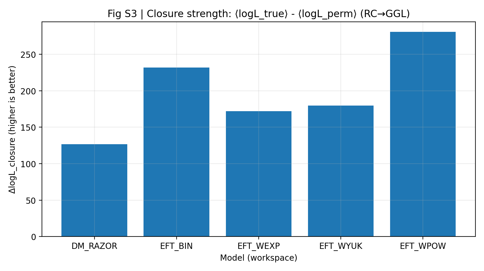
Figure S3 | Closure Strength (larger is better): Mean log-likelihood advantage for RC-only → GGL prediction.
How to Read This Figure |
This figure is the core of P1. The taller the bar, the better the information learned from RC transfers to GGL. |
The EFT family is overall higher than DM_RAZOR, indicating stronger EFT cross-probe closure in the “learn RC first, then predict GGL” experiment. |
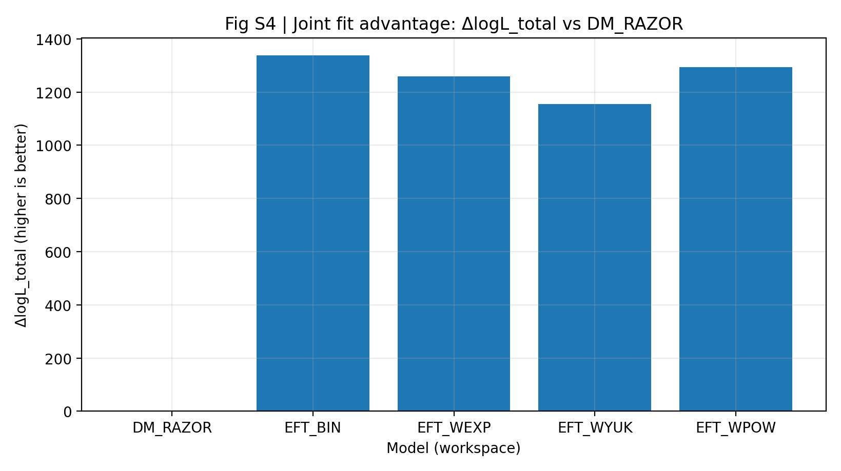
Figure S4 | Joint-Fit Advantage (larger is better): RC+GGL best logL_total relative to DM_RAZOR.
How to Read This Figure |
This figure shows the total score after RC and GGL are combined. |
All EFT models are well above 0, indicating that the EFT advantage in the main comparison is not a local single-point effect but an overall pattern in the joint analysis. |
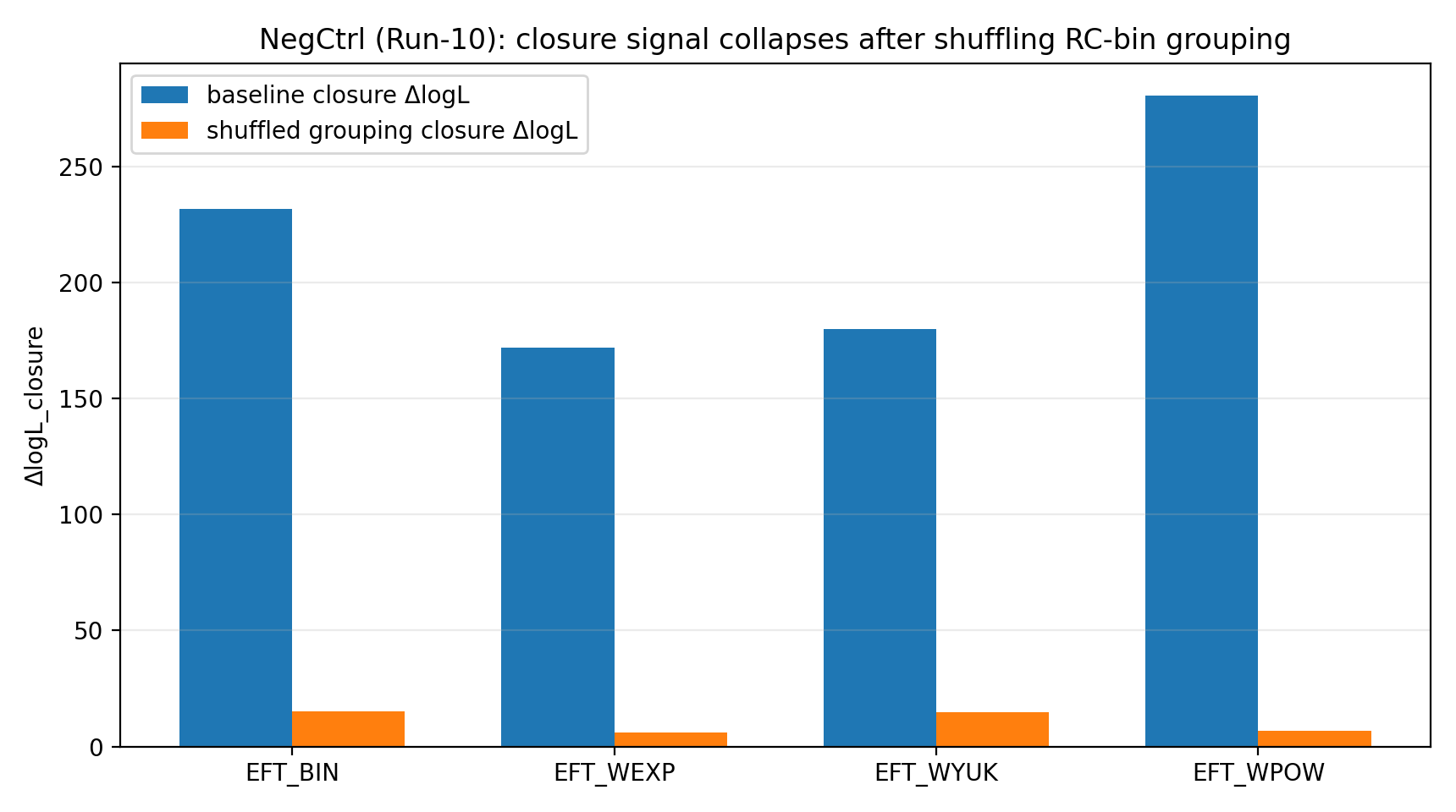
Figure R1 | Negative Control: Closure Signal Drops Sharply After Shuffling the Grouping.
How to Read This Figure |
This figure shows that once the correct RC↔GGL binning relationship is disrupted, the closure signal drops sharply. |
This makes the P1 result look more like genuine consistency in cross-data mapping, rather than a numerical coincidence obtainable under arbitrary mappings. |
8 | Robustness and Controls: How Does P1 Avoid Being “Just a Good-Looking Fit”?
The easiest challenge to raise against a technical report is whether the advantage comes from one noise setting, one central-region data cut, one covariance treatment, or overfitting. P1 addresses this with multiple stress tests.
Table 2 | How to Read P1’s Robustness Tests and Negative Controls
Test | Concern It Tries to Rule Out | How to Read It |
σ_int scan | If RC contains additional unknown scatter, does the conclusion remain stable? | After RC errors are relaxed, the EFT ranking and advantage scale remain stable. |
R_min scan | If the galaxy central regions are not fully trusted, does the conclusion remain stable? | After trimming the central regions, EFT still maintains a positive advantage. |
cov-shrink scan | If the GGL covariance estimate is uncertain, does the conclusion remain stable? | After covariance shrinkage toward the diagonal, the advantage is not sensitive. |
Ablation ladder | Is EFT relying on unnecessary complexity to force a fit? | The full EFT_BIN is supported by the information criteria. |
LOO held-out prediction | Does the model only explain data it has already seen? | After holding out a GGL bin, the model still shows strong generalization performance. |
RC-bin shuffle | Does closure come from the true mapping? | Closure drops after shuffling the grouping, supporting mapping dependence. |
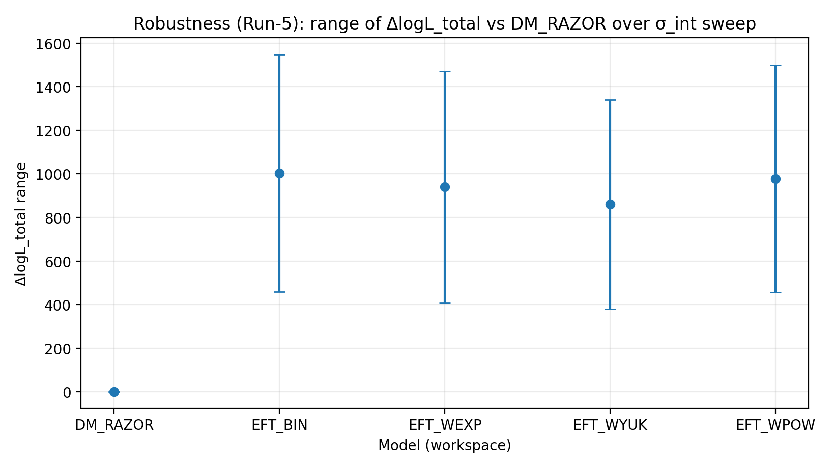
Figure R2 | Range of ΔlogL_total Under the σ_int Scan (larger is better).
How to Read This Figure |
Tests whether EFT’s lead remains after changes in the assumed intrinsic RC scatter. |
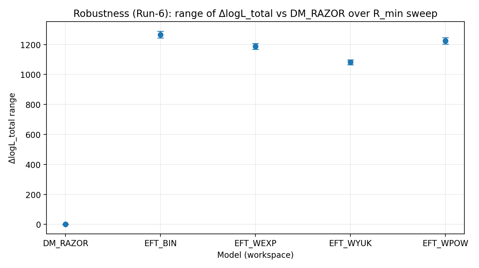
Figure R3 | Range of ΔlogL_total Under the R_min Scan (larger is better).
How to Read This Figure |
Tests whether EFT’s advantage remains stable after complex central regions are trimmed. |
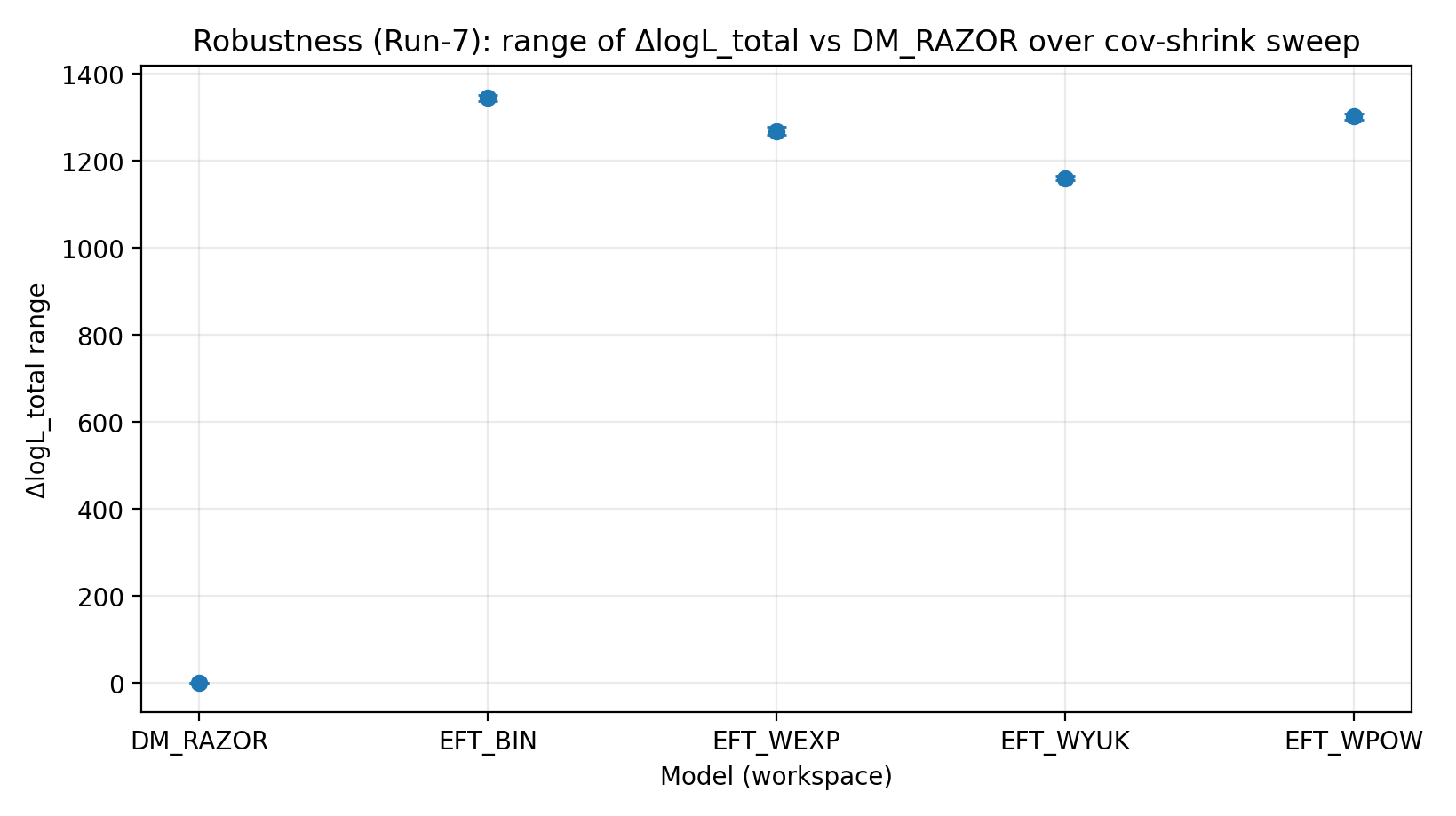
Figure R4 | Range of ΔlogL_total Under the cov-shrink Scan (larger is better).
How to Read This Figure |
Tests whether the ranking is sensitive to changes in weak-lensing covariance treatment. |
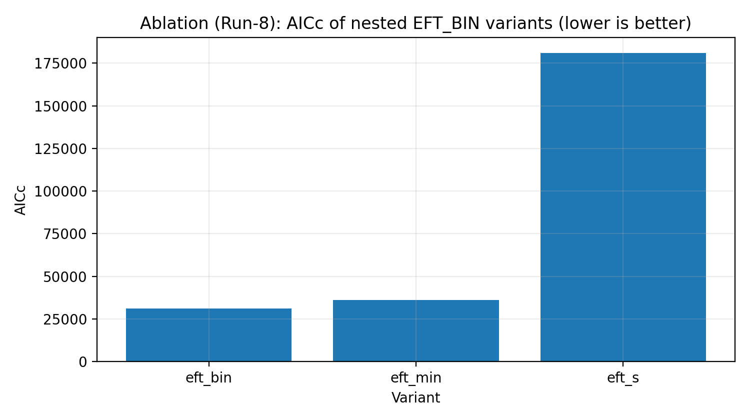
Figure R5 | EFT_BIN Ablation Ladder (AICc, smaller is better).
How to Read This Figure |
Tests whether the full EFT_BIN is necessary for explaining the data, rather than merely adding needless parameters. |
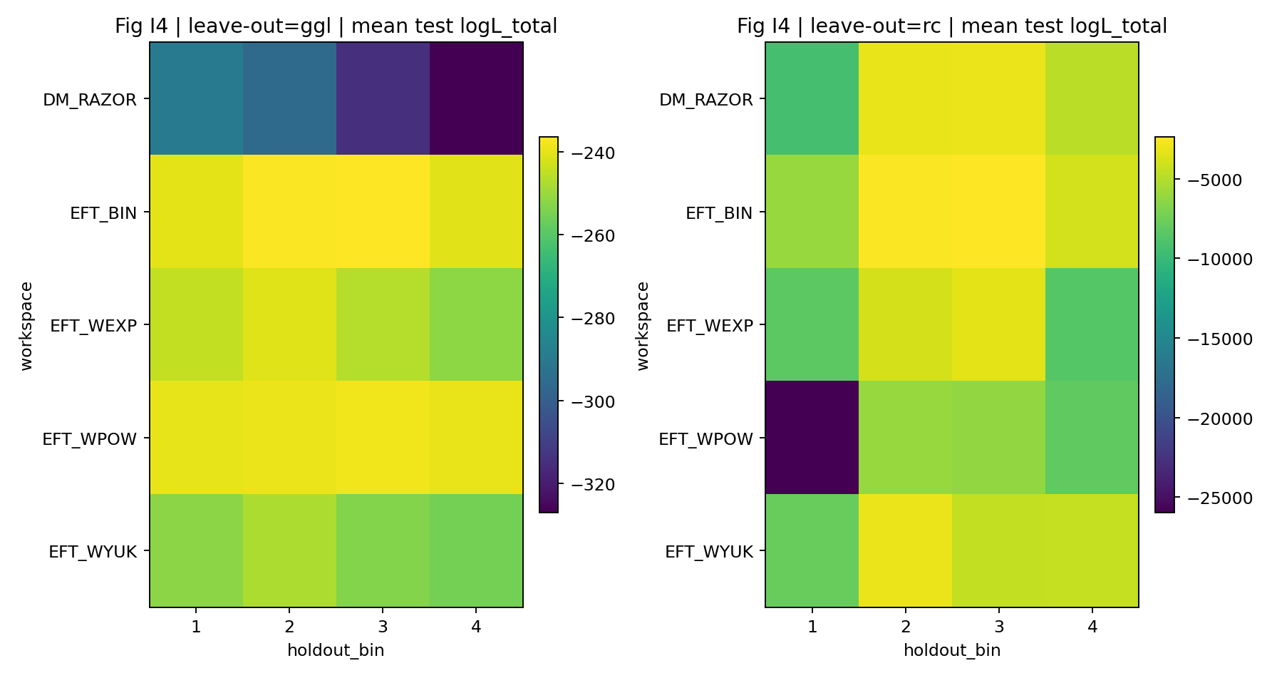
Figure R6 | LOO: Log-Likelihood Distribution for Held-Out Bins.
How to Read This Figure |
Tests whether the model still has predictive performance on unseen GGL bins. |
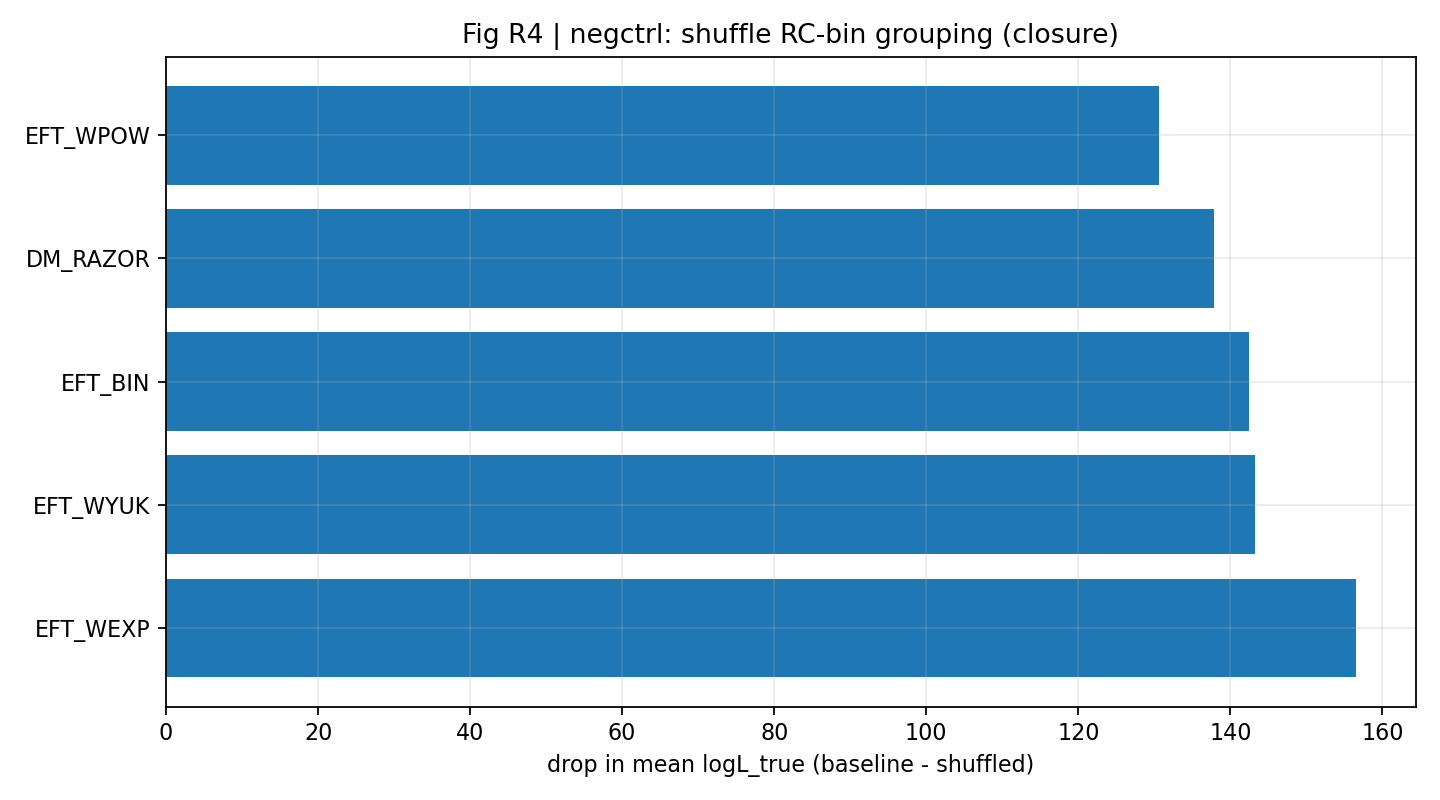
Figure R7 | Negative Control: Shuffled Mapping Causes a Clear Drop in Closure mean logL_true.
How to Read This Figure |
Further shows, from the perspective of mean logL_true, that closure depends on the correct cross-data mapping. |
9 | P1A: Why “Multiple DM Models in the Appendix” Is a Key Correction
This section is not asking, “Did EFT only beat one minimal DM_RAZOR baseline?” It asks whether the closure-test and joint-fit conclusions change when the DM baseline is strengthened within a low-dimensional, reproducible, clearly recorded parameter ledger (P1A). In other words, P1A aims to reduce the objection that “you merely chose an overly weak DM baseline” and moves the discussion toward whether closure behavior still differs under a set of auditable DM enhancements.
P1A is not designed to exhaust all possible LambdaCDM halo modeling, nor does it turn the DM side into a high-dimensional, unauditable fitter. It selects low-dimensional, reproducible enhancements with a clear parameter ledger: concentration scatter, adiabatic contraction, feedback core, hierarchical c–M scatter prior, one-parameter core proxy, weak-lensing shear-calibration nuisance, and the combined DM_STD baseline.
Main Reading of P1A |
Among the three legacy branches, only feedback/core produces a small net increase in closure strength; SCAT and AC do not produce net closure gains. |
DM_HIER_CMSCAT, DM_RAZOR_M, and DM_CORE1P have very little effect on closure strength or do not show a significant net improvement. |
DM_STD can substantially improve joint logL, but its closure strength decreases, suggesting that it mainly improves joint-fit flexibility rather than RC→GGL transfer-prediction power. |
EFT_BIN still retains higher closure strength and a joint-fit advantage in P1A Table B1; therefore, P1’s core claim should not be reduced to “it only beat minimal DM_RAZOR.” |
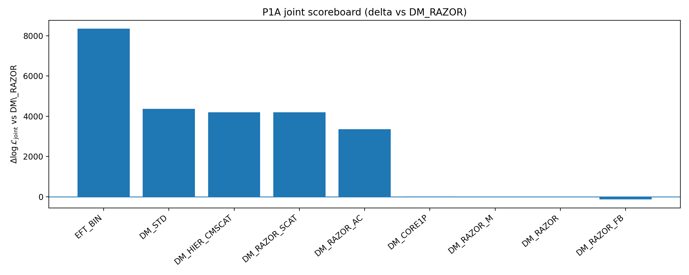
Figure B1 | P1A Scoreboard: Closure and Joint ΔlogL Relative to Baseline (larger is better).
How to Read This Figure |
This figure shows the performance of multiple DM enhancement branches relative to the baseline. |
Its meaning is not “all DM is excluded,” but rather this: within the low-dimensional, auditable DM enhancements selected by P1A, strengthening DM does not remove EFT_BIN’s closure advantage. |
10 | Why the P1 Experiment Matters
10.1 Methodological Significance: Placing “Cross-Probe Closure” Above “Single-Probe Fitting”
Galaxy-scale theory can easily get stuck on whether a model can fit a particular set of rotation curves. P1 raises the question one level: can parameters learned from RC predict weak lensing without retuning to GGL? This turns P1 from a “fitting contest” into a “transfer-prediction test.”
10.2 Transparency Significance: Treating the Reproducibility Chain as Part of the Result
One important contribution of P1 is that it releases the data, tables and figures, run labels, negative controls, reproduction package, and audit chain together. This matters for both supporters and critics: discussion can return to the same public data, the same mapping, the same scripts, and the same metrics, rather than comparing slogans.
10.3 Physical Significance: A Strong Stress Test for “Non-Dark-Matter Gravity” Directions
In non-dark-matter gravity directions, many models can explain some part of rotation curves or the RAR. The harder task is to also pass weak-lensing readouts and show under negative controls that the signal depends on the correct mapping. P1 matters because it places EFT mean gravitational response into a protocol like an external examination: RC is the training ground, GGL is the transfer field, and shuffle is the anti-cheating field.
10.4 Is This an Important Experiment for the “Non-Dark-Matter Gravity” Field?
Carefully stated: if P1’s data processing, reproduction package, and closure protocol hold up under external review, then it can be regarded as an RC+GGL closure experiment worth taking seriously in non-dark-matter gravity / modified-gravity directions. Its importance does not lie in the slogan “dark matter is overturned,” but in providing a cross-probe criterion that can be replicated, challenged, and extended.
Are There Already RC+GGL Prediction-Closure Frameworks at the Same Level? |
There are relevant frameworks and observational traditions: MOND/RAR organizes many rotation-curve phenomena well; the KiDS-1000 weak-lensing RAR work also compared MOND, Verlinde emergent gravity, and LambdaCDM models; LambdaCDM can also explain some weak-lensing/dynamical phenomena through galaxy–halo connections, gas halos, and feedback modeling. |
But P1’s precise claim is not that “no other framework in the world can explain RC+GGL.” Rather, under P1’s own public protocol—fixed mapping, RC-only→GGL closure, shuffle negative controls, parameter ledger, and P1A multi-DM stress tests—EFT reports stronger closure performance. |
In other words, the part of P1 most worth external testing is its concrete, reproducible comparison protocol. A very worthwhile next step is to see whether MOND/RAR, LambdaCDM/HOD, hydrodynamical simulations, or other modified-gravity frameworks can reach the same or higher closure scores under the same protocol. |
11 | What Can P1 Conclude, and What Can It Not Conclude?
Table 3 | Boundaries of P1’s Conclusions
Can Conclude | Under P1’s RC+GGL data, fixed mapping, and main comparison protocol, the EFT family has higher joint-fit scores and closure strength than the minimal DM_RAZOR. |
Can Conclude | Within P1A’s low-dimensional, auditable DM-enhancement range, multiple DM enhancements do not eliminate EFT_BIN’s closure advantage. |
Can Conclude | The shuffle negative control shows that the closure signal depends on the correct cross-data mapping and is not obtainable under arbitrary mappings. |
Cannot Conclude | One cannot say that P1 has overturned all dark-matter models. P1A still does not exhaust non-sphericity, environmental dependence, complex galaxy–halo connections, high-dimensional feedback, or full cosmological simulations. |
Cannot Conclude | One cannot say that the complete EFT framework has been proven from first principles. P1 tests only the phenomenological layer of mean gravitational response. |
Cannot Conclude | One cannot say that all systematics have been ruled out. P1 provides robustness evidence only within the listed stress tests and audit scope. |
12 | Frequently Asked Questions from General Readers
Q1: Is this saying that “dark matter does not exist”?
No. P1’s conclusions must be limited to the data, protocol, and comparison models used here. P1A goes beyond the minimal DM_RAZOR, but it still does not represent all possible dark-matter models.
Q2: Is this saying that “EFT has been proven”?
Also no. P1 tests EFT as a parameterization of mean gravitational response and shows stronger performance in RC→GGL closure; the microscopic mechanism and complete theory are not P1’s conclusion.
Q3: Why not report a significance value in σ directly?
P1 uses unified likelihood scores, information criteria, and closure differences. ΔlogL is a relative advantage under the same scoring rule; it is not equivalent to a single σ value.
Q4: Why shuffle RC-bin→GGL-bin?
This is a negative control. A real cross-probe signal should depend on the correct mapping; if it remains just as strong after shuffling, that would instead suggest possible implementation bias or a statistical false signal.
Q5: What should P1 do next?
Extend the same protocol to more data, more DM comparisons, more complex systematics, and more modified-gravity frameworks—especially in ways that allow external teams to retest under the same closure metric.
13 | Mini Glossary
Table 4 | Mini Glossary
Term | One-Sentence Explanation |
Rotation curve (RC) | The radius–rotation-speed relation in a galaxy disk, used to infer effective gravity within the disk. |
Weak lensing (GGL) | A measure of the average gravitational/mass distribution around foreground galaxies through the statistical distortion of background galaxy shapes. |
Closure test | Uses the RC posterior to predict GGL, then compares it with the negative control produced by shuffled mapping. |
Negative control | Deliberately breaks a key structure to see whether the signal disappears; used to rule out false signals. |
NFW halo | A dark-matter-halo density profile commonly used in cold-dark-matter models. |
c–M relation | The relation between dark-matter-halo concentration c and mass M; whether scatter is allowed affects model flexibility. |
DM_STD | The standardized DM stress-test branch in P1A that combines multiple low-dimensional DM enhancements and a lensing nuisance term. |
ΔlogL | The log-likelihood difference between two models under the same scoring rule; a positive value means the former is better. |
Covariance | A matrix description of correlations among data points; weak-lensing data usually require the full covariance. |
14 | Suggested Reading Path and Citation Entry Points
1. First read Sections 0–2 of this guide to establish P1’s question and EFT’s deliberately restrained role in P1.
2. Then read Figure S3, Figure S4, and Tables S1a/S1b to understand closure strength, joint fitting, and negative controls.
3. If you are concerned that the “DM baseline is too weak,” go directly to Section 9 and Table B1 / Figure B1.
4. For technical verification, return to the P1 technical report v1.1, the Tables & Figures Supplement, and the full_fit_runpack.
Main Archive Entry Points |
P1 technical report (release-level, Concept DOI): 10.5281/zenodo.18526334 |
P1 full reproduction package (Concept DOI): 10.5281/zenodo.18526286 |
EFT structured knowledge base (optional, Concept DOI): 10.5281/zenodo.18853200 |
License note: the technical report uses CC BY-NC-ND 4.0; the full reproduction package uses CC BY 4.0 (refer to the technical report and Zenodo archives as authoritative). |
15 | References and External Background
McGaugh, S. S., Lelli, F., & Schombert, J. M. (2016). The Radial Acceleration Relation in Rotationally Supported Galaxies. Physical Review Letters, 117, 201101. DOI: 10.1103/PhysRevLett.117.201101.
Famaey, B., & McGaugh, S. S. (2012). Modified Newtonian Dynamics (MOND): Observational Phenomenology and Relativistic Extensions. Living Reviews in Relativity, 15, 10. DOI: 10.12942/lrr-2012-10.
Brouwer, M. M., Oman, K. A., Valentijn, E. A., et al. (2021). The weak lensing radial acceleration relation: Constraining modified gravity and cold dark matter theories with KiDS-1000. Astronomy & Astrophysics, 650, A113. DOI: 10.1051/0004-6361/202040108.
Mistele, T., McGaugh, S., Lelli, F., Schombert, J., & Li, P. (2024). Indefinitely Flat Circular Velocities and the Baryonic Tully-Fisher Relation from Weak Lensing. The Astrophysical Journal Letters, 969, L3 / arXiv:2406.09685.
Bullock, J. S., & Boylan-Kolchin, M. (2017). Small-Scale Challenges to the LambdaCDM Paradigm. Annual Review of Astronomy and Astrophysics, 55, 343–387. DOI: 10.1146/annurev-astro-091916-055313.
Lelli, F., McGaugh, S. S., & Schombert, J. M. (2016). SPARC: Mass Models for 175 Disk Galaxies with Spitzer Photometry and Accurate Rotation Curves. The Astronomical Journal, 152, 157. DOI: 10.3847/0004-6256/152/6/157.
Navarro, J. F., Frenk, C. S., & White, S. D. M. (1997). A Universal Density Profile from Hierarchical Clustering. Astrophysical Journal, 490, 493.
Dutton, A. A., & Macciò, A. V. (2014). Cold dark matter haloes in the Planck era: evolution of structural parameters for NFW haloes. Monthly Notices of the Royal Astronomical Society, 441, 3359–3374.